Advanced R - Notes (part1)
Advanced R (Hadley Wickham).
knitr::opts_chunk$set(error = TRUE)suppressPackageStartupMessages(library(tidyverse))
suppressPackageStartupMessages(library(rlang))
suppressPackageStartupMessages(library(lobstr))
suppressPackageStartupMessages(library(withr))
suppressPackageStartupMessages(library(glue))
# devtools::install_github("openpharma/simaerep@v0.3.1")
suppressPackageStartupMessages(library(simaerep))Functions
Conventions for arguments that come from a set of strings
center <- function(x, type = c("mean", "median", "trimmed")) {
  type <- match.arg(type)
  switch(type,
         mean = mean(x),
         median = median(x),
         trimmed = mean(x, trim = .1))
}
Functions to Investigate Functions
.f <- function(x,y){
  # Comment
  x + y
}
formals(.f) # returns arguments
## $x
##
##
## $ybody(.f) # returns body without comments## {
## x + y
## }environment(.f) ## <environment: R_GlobalEnv>attributes(.f)$srcref # returns body with commments## function(x,y){
## # Comment
## x + y
## }Get all Functions from package
objs <- mget(ls("package:base", all = TRUE), inherits = TRUE)
funs <- Filter(is.function, objs)
Function with the most arguments
primitive base functions written in C are either of type “builtin” or “special”. formals(), body()and environment() will return NULL for those functions.
df_funs <- tibble(funs = funs,
       names = names(funs) ) %>%
  mutate(formals = map(funs, formals),
         n_args = map_int(formals, length),
         type = map_chr(funs, typeof)) %>%
  arrange(desc(n_args))

df_funs
## # A tibble: 1,323 × 5
## funs names formals n_args type
## <named list> <chr> <named list> <int> <chr>
## 1 <fn> scan <pairlist> 22 closure
## 2 <fn> format.default <pairlist> 16 closure
## 3 <fn> source <pairlist> 16 closure
## 4 <fn> formatC <pairlist> 15 closure
## 5 <fn> library <pairlist> 13 closure
## 6 <fn> merge.data.frame <pairlist> 13 closure
## 7 <fn> prettyNum <pairlist> 13 closure
## 8 <fn> system2 <pairlist> 11 closure
## 9 <fn> print.default <pairlist> 10 closure
## 10 <fn> save <pairlist> 10 closure
## # … with 1,313 more rowsdf_funs %>%
group_by(type, n_args == 0) %>%
count()## # A tibble: 4 × 3
## # Groups: type, n_args == 0 [4]
## type `n_args == 0` n
## <chr> <lgl> <int>
## 1 builtin TRUE 165
## 2 closure FALSE 1072
## 3 closure TRUE 47
## 4 special TRUE 39Scoping
Search Environment
my_string <- "hello world"

exists("my_string")
## [1] TRUEexists("my_string_2")## [1] FALSEget0("my_string")## [1] "hello world"get0("my_string_2")## NULLls() # get all variable names## [1] "center" "df_funs" "funs" "my_string" "objs"List unbound global variables
g12 <- function() x + 1
codetools::findGlobals(g12)
## [1] "+" "x"g13 <- function(x) x + 1
codetools::findGlobals(g13)## [1] "+"Lazy Evaluation of Arguments
arguments even when given as expressions will only be evaluated when called in the function, these structures are called promises. So this works, surprisingly:
h04 <- function(x = 1, y = x * 2, z = a + b) {
  a <- 10
  b <- 100

  c(x, y, z)
}
But only when supplied as default arguments not when user-supplied
h04(1, x * 2, a + b)## Error in h04(1, x * 2, a + b): object 'x' not foundUser-Supplied arguments are evaluated before they are passed to the function, that is why infix functions and operators such as + and %%are working.
Default arguments are evaluated as promises only when they are called within the function.
Reminder infix functions take two arguments, code that comes directly before and right after. User defined infix functions need to be defined like this with `%name% <- function(lhs, rhs)`
x <- 1

!is.null(x) && length(x) == 1 && x > 0
## [1] TRUE# in python we would need to put brackets around the logic statements
(!is.null(x)) && (length(x) == 1) && (x > 0)## [1] TRUEc(TRUE, FALSE) && c(TRUE, FALSE) # evaluation stops at first element## [1] TRUEc(TRUE, FALSE) & c(TRUE, FALSE) # all elements are pair-wise evaluated## [1] TRUE FALSEFALSE && NULL # evaluation stops after result is determined by first argument FALSE## [1] FALSEFALSE || NULL # gives error because NULL needs to be evaluated for OR condition## Error in FALSE || NULL: invalid 'y' type in 'x || y'FALSE & NULL # I would expect this to error too## logical(0)FALSE | NULL # this as well mmh## logical(0)Default or User Supplied argument
h06 <- function(x = 10) {
  is_default <- missing(x)
  return(is_default)
}

h06()
## [1] TRUEh06(10)## [1] FALSECapture dot dot dot
i03 <- function(...) {
  list(first = ..1, third = ..3)
}
str(i03(1, 2, 3))
## List of 2
## $ first: num 1
## $ third: num 3i04 <- function(...) {
list(...)
}
str(i04(a = 1, b = 2))## List of 2
## $ a: num 1
## $ b: num 2Exit Handler on.exit()
Always set add = TRUE when using on.exit(). If you don’t, each call to on.exit() will overwrite the previous exit handler. Even when only registering a single handler, it’s good practice to set add = TRUE so that you won’t get any unpleasant surprises if you later add more exit handlers.
j06 <- function(x) {
  cat("Hello\n")
  on.exit(cat("Goodbye!\n"), add = TRUE)

  if (x) {
    return(10)
  } else {
    stop("Error")
  }
}

j06(TRUE)
## Hello
## Goodbye!## [1] 10j06(FALSE)## Hello## Error in j06(FALSE): Error## Goodbye!Better than using on.exit is actually to use functions of the withr package that automatically provide cleanups for files and directories
Capture output capture.output()
also captures error messages
Everything that happens in R is a function call
Almost everything can be rewritten as a function call
x + y## Error in eval(expr, envir, enclos): object 'y' not found`+`(x, y)## Error in eval(expr, envir, enclos): object 'y' not foundnames(df) <- c("x", "y", "z")## Error in names(df) <- c("x", "y", "z"): names() applied to a non-vector`names<-`(df, c("x", "y", "z"))## Error in eval(expr, envir, enclos): names() applied to a non-vectorfor(i in 1:10) print(i)## [1] 1
## [1] 2
## [1] 3
## [1] 4
## [1] 5
## [1] 6
## [1] 7
## [1] 8
## [1] 9
## [1] 10`for`(i, 1:10, print(i))## [1] 1
## [1] 2
## [1] 3
## [1] 4
## [1] 5
## [1] 6
## [1] 7
## [1] 8
## [1] 9
## [1] 10Replacement Functions
`second<-` <- function(x, value) {
  x[2] <- value
  x
}

x <- 1:10
second(x) <- 5

x
## [1] 1 5 3 4 5 6 7 8 9 10Environments
Generally, an environment is similar to a named list, with four important exceptions:
- Every name must be unique.
- The names in an environment are not ordered.
- An environment has a parent.
- Environments are not copied when modified.
e1 <- env(
  a = FALSE,
  b = "a",
  c = 2.3,
  d = 1:3,
)

rlang::env_print(e1)
## <environment: 0x7fd2d346bac0>
## parent: <environment: global>
## bindings:
## * a: <lgl>
## * b: <chr>
## * c: <dbl>
## * d: <int>rlang::env_names(e1)## [1] "a" "b" "c" "d"Create a parent environment
e2 <- env(e1, letters = LETTERS)

rlang::env_parent(e2)
## <environment: 0x7fd2d346bac0>rlang::env_parents(e2)## [[1]] <env: 0x7fd2d346bac0>
## [[2]] $ <env: global>Packages
Composition of the global environment
search()## [1] ".GlobalEnv" "package:simaerep" "package:glue"
## [4] "package:withr" "package:lobstr" "package:rlang"
## [7] "package:forcats" "package:stringr" "package:dplyr"
## [10] "package:purrr" "package:readr" "package:tidyr"
## [13] "package:tibble" "package:ggplot2" "package:tidyverse"
## [16] "package:stats" "package:graphics" "package:grDevices"
## [19] "package:utils" "package:datasets" "package:methods"
## [22] "Autoloads" "package:base"rlang::search_envs()## [[1]] $ <env: global>
## [[2]] $ <env: package:simaerep>
## [[3]] $ <env: package:glue>
## [[4]] $ <env: package:withr>
## [[5]] $ <env: package:lobstr>
## [[6]] $ <env: package:rlang>
## [[7]] $ <env: package:forcats>
## [[8]] $ <env: package:stringr>
## [[9]] $ <env: package:dplyr>
## [[10]] $ <env: package:purrr>
## [[11]] $ <env: package:readr>
## [[12]] $ <env: package:tidyr>
## [[13]] $ <env: package:tibble>
## [[14]] $ <env: package:ggplot2>
## [[15]] $ <env: package:tidyverse>
## [[16]] $ <env: package:stats>
## [[17]] $ <env: package:graphics>
## [[18]] $ <env: package:grDevices>
## [[19]] $ <env: package:utils>
## [[20]] $ <env: package:datasets>
## ... and 3 more environmentsPackage Functions
- passively bound by one environment (where they can be called from)
- actively bind one environment (which they use to make their calls)
for regular functions both environments are the same. For functions loaded from packages the bind environment is defined by the package namespace created from the package NAMESPACE file. Like this they are not affected by overrides in the execution environment.
Callstacks
use lobstr::cst() in a similar way to traceback() to visualise the callstack.
f <- function(x) {
  g(x = 2)
}
g <- function(x) {
  h(x = 3)
}
h <- function(x) {
  stop()
}

f(x = 1)
## Error in h(x = 3):traceback()## No traceback availableh <- function(x) {
lobstr::cst()
print("do I get executed =")
}
f(x = 1)## █
## 1. └─global::f(x = 1)
## 2. └─global::g(x = 2)
## 3. └─global::h(x = 3)
## 4. └─lobstr::cst()
## [1] "do I get executed ="Conditions
Warnings
give_warning <- function() {
  warning("You have been warned")
}

withr::with_options(list(warn = 1), give_warning()) # causes warning to appear immediately
## Warning in give_warning(): You have been warnedwithr::with_options(list(warn = 2), give_warning()) # convert warning to error## Error in give_warning(): (converted from warning) You have been warnedCondition Objects
conditions such as messages, warnings and errors are objects
cnd <- rlang::catch_cnd(stop("An error"))
str(cnd)
## List of 2
## $ message: chr "An error"
## $ call : language force(expr)
## - attr(*, "class")= chr [1:3] "simpleError" "error" "condition"tryCatch
tryCatch executes code and has arguments for different types of condition objects. Each arguments takes a function with a single condition object argument.
try_me <- function(expr) {
    tryCatch(
      error = function(cnd) print("error"),
      warning = function(cnd) print("warning"),
      message = function(cnd) print("message"),
      finally = print("finished"),
      expr
  )
}

try_me(stop("hello"))
## [1] "error"
## [1] "finished"try_me(warning("hello"))## [1] "warning"
## [1] "finished"try_me(message("hello"))## [1] "message"
## [1] "finished"variable assignments within trycatch are not passed to parent env
if(exists("res")) remove(res)
tryCatch(
  warning = function(cnd) res <- 0,
  res <- log(-1)
)
exists("res")
## [1] FALSEthis does not work because user-defined arguments are evaluated on the spot, so alternative expression always gets evaluated
try_me3 <- function(expr, expr_alt) {
    tryCatch(
      warning = function(cnd) expr_alt,
      expr
  )
}

try_me3(res <- log(-1), res <- 0)
res
## [1] 0try_me3(res <- log(1), res <- 0)
res## [1] 0tryCatch returns last value which can be assigned inside the active env
if(exists("res")) remove(res)
res <- tryCatch(
  warning = function(cnd) 0,
  log(-1)
)

res
## [1] 0withCallingHandlers
withCallingHandlers still executes the condition, while tryCatch muffles them.
try_me <- function(expr) {
    withCallingHandlers(
      error = function(cnd) print("error"),
      warning = function(cnd) print("warning"),
      message = function(cnd) print("message"),
      finally = print("finished"),
      expr
  )
}

try_me(stop("hello"))
## [1] "finished"
## [1] "error"## Error in withCallingHandlers(error = function(cnd) print("error"), warning = function(cnd) print("warning"), : hellotry_me(warning("hello"))## [1] "finished"
## [1] "warning"## Warning in withCallingHandlers(error = function(cnd) print("error"), warning =
## function(cnd) print("warning"), : hellotry_me(message("hello"))## [1] "finished"
## [1] "message"## helloCustom Errors
- reuse check function to supply consistent error messages
- catch and handle different types of errors
We start by defining a custom error Class
We cannot execute the code chunk below because Rmarkdown is not compatible with custom errors
stop_custom <- function(.subclass, message, ...) {
  err <- structure(
    list(
      message = message,
      call = call,
      ...
    ),
    class = c(.subclass, "error", "condition")
  )
  stop(err)
}

stop_custom("error_new", "This is a custom error", x = 10)

err <- rlang::catch_cnd(
  stop_custom("error_new", "This is a custom error", x = 10)
)

class(err)
# we can supply additional arguments that will be attached as attributes
err$x
str(err)
We can then use this new class for creating customized errors
abort_bad_argument <- function(arg, must, not = NULL) {
  msg <- glue::glue("`{arg}` must be {must}")
  if (!is.null(not)) {
    not <- typeof(not)
    msg <- glue::glue("{msg}; not {not}.")
  }

  stop_custom("error_bad_argument",
    message = msg,
    arg = arg,
    must = must,
    not = not
  )
}

abort_bad_argument("key", "numeric", "ABC")
## Error in stop_custom("error_bad_argument", message = msg, arg = arg, must = must, : could not find function "stop_custom"We can then chose to handle those errors specifically
mylog <- function(x) {
  if(! is.numeric(x)) abort_bad_argument("x", "numeric", x)
  return(log(x))
}

mylog(1)
## [1] 0mylog("A")## Error in stop_custom("error_bad_argument", message = msg, arg = arg, must = must, : could not find function "stop_custom"tryCatch(
error_bad_argument = function(cnd) NULL,
mylog("A")
)## Error in stop_custom("error_bad_argument", message = msg, arg = arg, must = must, : could not find function "stop_custom"tryCatch(
error_bad_argument = function(cnd) NULL,
stop()
)## Error in doTryCatch(return(expr), name, parentenv, handler):Functional Programming
Functionals
purrr::reduce
used to apply a function with two arguments to a stack o items by executing on the first to items and saving the result for the next function call to apply with the next item in line.
purrr::reduce(LETTERS, paste0)## [1] "ABCDEFGHIJKLMNOPQRSTUVWXYZ"finding an intersection or union
l <- purrr::map(1:4, ~ sample(1:10, 15, replace = T))
str(l)
## List of 4
## $ : int [1:15] 5 5 1 9 6 9 1 8 4 4 ...
## $ : int [1:15] 7 3 4 5 2 6 5 9 9 8 ...
## $ : int [1:15] 1 3 3 7 1 8 10 1 4 10 ...
## $ : int [1:15] 8 7 7 7 5 6 5 8 5 7 ...purrr::reduce(l, intersect)## [1] 8 4 2purrr::reduce(l, union)## [1] 5 1 9 6 8 4 2 7 3 10adding up numbers
purrr::reduce(c(1, 2, 3), `+`)## [1] 6purrr::accumulate
purrr::accumulate(LETTERS, paste0)## [1] "A" "AB"
## [3] "ABC" "ABCD"
## [5] "ABCDE" "ABCDEF"
## [7] "ABCDEFG" "ABCDEFGH"
## [9] "ABCDEFGHI" "ABCDEFGHIJ"
## [11] "ABCDEFGHIJK" "ABCDEFGHIJKL"
## [13] "ABCDEFGHIJKLM" "ABCDEFGHIJKLMN"
## [15] "ABCDEFGHIJKLMNO" "ABCDEFGHIJKLMNOP"
## [17] "ABCDEFGHIJKLMNOPQ" "ABCDEFGHIJKLMNOPQR"
## [19] "ABCDEFGHIJKLMNOPQRS" "ABCDEFGHIJKLMNOPQRST"
## [21] "ABCDEFGHIJKLMNOPQRSTU" "ABCDEFGHIJKLMNOPQRSTUV"
## [23] "ABCDEFGHIJKLMNOPQRSTUVW" "ABCDEFGHIJKLMNOPQRSTUVWX"
## [25] "ABCDEFGHIJKLMNOPQRSTUVWXY" "ABCDEFGHIJKLMNOPQRSTUVWXYZ"predicate functional
purr has only some of those
any(LETTERS == "A")## [1] TRUEany(as.list(LETTERS) == "A")## [1] TRUEpurrr::some(LETTERS, ~ . == "A")## [1] TRUEis.na
is.na() is not a predicate function because it is vectorized while anyNA is.
is.na(c(NA, 1))## [1] TRUE FALSEanyNA(c(NA, 1))## [1] TRUEapply() and friends
vapply()uses and returns vectorssapply()
ls <- list(a = c(1, 2, 3), b = c(TRUE, FALSE, TRUE, FALSE))
vs <- c("do", "not", "leak")
cl <- structure(ls, class = "apply_test")
purrr::map() is similar to base::lapply() which uses lists as in and output.
purrr::map(ls, sum)## $a
## [1] 6
##
## $b
## [1] 2purrr::map(vs, str_length)## [[1]]
## [1] 2
##
## [[2]]
## [1] 3
##
## [[3]]
## [1] 4purrr::map(ls, sum)## $a
## [1] 6
##
## $b
## [1] 2lapply(ls, sum)## $a
## [1] 6
##
## $b
## [1] 2lapply(vs, str_length)## [[1]]
## [1] 2
##
## [[2]]
## [1] 3
##
## [[3]]
## [1] 4lapply(cl, sum)## $a
## [1] 6
##
## $b
## [1] 2sapply() is more flexible and returns vectors if possible
sapply(ls, sum)## a b
## 6 2sapply(vs, str_length)## do not leak
## 2 3 4sapply(cl, sum)## a b
## 6 2vapply() is similar to sapply() requires a FUN.Value argument to set requirements for the output.
It compares the length and type of the FUN.Value argument with the output.
vapply(ls, sum)## Error in vapply(ls, sum): argument "FUN.VALUE" is missing, with no defaultvapply(ls, sum, FUN.VALUE = integer(1))## Error in vapply(ls, sum, FUN.VALUE = integer(1)): values must be type 'integer',
## but FUN(X[[1]]) result is type 'double'vapply(ls, sum, FUN.VALUE = double(1))## a b
## 6 2vapply(ls, sum, FUN.VALUE = double(2))## Error in vapply(ls, sum, FUN.VALUE = double(2)): values must be length 2,
## but FUN(X[[1]]) result is length 1vapply(ls, sum, FUN.VALUE = c(c = 8))## a b
## 6 2vapply(ls, sum, FUN.VALUE = "hello")## Error in vapply(ls, sum, FUN.VALUE = "hello"): values must be type 'character',
## but FUN(X[[1]]) result is type 'double'vapply(vs, str_length, 9999)## do not leak
## 2 3 4vapply(cl, sum, 1)## a b
## 6 2sapply() can also return a matrix
i39 <- sapply(3:9, seq)
i39
## [[1]]
## [1] 1 2 3
##
## [[2]]
## [1] 1 2 3 4
##
## [[3]]
## [1] 1 2 3 4 5
##
## [[4]]
## [1] 1 2 3 4 5 6
##
## [[5]]
## [1] 1 2 3 4 5 6 7
##
## [[6]]
## [1] 1 2 3 4 5 6 7 8
##
## [[7]]
## [1] 1 2 3 4 5 6 7 8 9# fivenum returns boxcox stats
x <- fivenum(i39[[1]])
vapply(vs, str_length)## Error in vapply(vs, str_length): argument "FUN.VALUE" is missing, with no defaultvapply(cl, sum)## Error in vapply(cl, sum): argument "FUN.VALUE" is missing, with no defaultlapply(i39, fivenum)## [[1]]
## [1] 1.0 1.5 2.0 2.5 3.0
##
## [[2]]
## [1] 1.0 1.5 2.5 3.5 4.0
##
## [[3]]
## [1] 1 2 3 4 5
##
## [[4]]
## [1] 1.0 2.0 3.5 5.0 6.0
##
## [[5]]
## [1] 1.0 2.5 4.0 5.5 7.0
##
## [[6]]
## [1] 1.0 2.5 4.5 6.5 8.0
##
## [[7]]
## [1] 1 3 5 7 9sapply(i39, fivenum)## [,1] [,2] [,3] [,4] [,5] [,6] [,7]
## [1,] 1.0 1.0 1 1.0 1.0 1.0 1
## [2,] 1.5 1.5 2 2.0 2.5 2.5 3
## [3,] 2.0 2.5 3 3.5 4.0 4.5 5
## [4,] 2.5 3.5 4 5.0 5.5 6.5 7
## [5,] 3.0 4.0 5 6.0 7.0 8.0 9vapply() can add row_names
vapply(i39, fivenum,
       c(Min. = 0, "1st Qu." = 0, Median = 0, "3rd Qu." = 0, Max. = 0))
## [,1] [,2] [,3] [,4] [,5] [,6] [,7]
## Min. 1.0 1.0 1 1.0 1.0 1.0 1
## 1st Qu. 1.5 1.5 2 2.0 2.5 2.5 3
## Median 2.0 2.5 3 3.5 4.0 4.5 5
## 3rd Qu. 2.5 3.5 4 5.0 5.5 6.5 7
## Max. 3.0 4.0 5 6.0 7.0 8.0 9vapply(i39, fivenum,
c(Min. = 0, "1st Qu." = 0, Median = 0, "3rd Qu." = 0))## Error in vapply(i39, fivenum, c(Min. = 0, `1st Qu.` = 0, Median = 0, `3rd Qu.` = 0)): values must be length 4,
## but FUN(X[[1]]) result is length 5Function Factories
Functions that return other functions. Those functions are not garbage collectd and need to be deleted manually.
force()
The expression are evaluated lazily thus when x changes the function does not behave as expected.
power <- function(exp) {
  function(x) {
    x ^ exp
  }
}

x <- 2
square <- power(x)
x <- 3
square(2)
## [1] 8always use force() when creating function factories
power2 <- function(exp) {
  force(exp)
  function(x) {
    x ^ exp
  }
}

x <- 2
square <- power2(x)
x <- 3
square(2)
## [1] 4Closures (Stateful functions)
not recommended in R
storer <- function(){
  store_var <- 5
  function() store_var
}
storage <- storer()
storage()
## [1] 5exists("store_var", envir = rlang::current_env())## [1] FALSEexists("store_var", envir = environment(storage))## [1] TRUEmake_counter <- function(){
count_var <- 0
function() {
count_var <<- count_var + 1 # <<- passes the assignment to parent environment where it is preserved via the binding
count_var
}
}
counter <- make_counter()
exists("count_var", envir = rlang::current_env())## [1] FALSEexists("count_var", envir = environment(counter))## [1] TRUEcounter()## [1] 1counter()## [1] 2counter()## [1] 3counter()## [1] 4Applications
stats::approxfun()stats::ecdf()scales::comma_format()and otherscalesfunctionsgeom_histogram()binwidth argument (see below)- harmonising input arguments of similar functions
- Box-Cox Transformation (see below)
- Bootstrap Resampling (see below)
- Maximum Likelihood Estimation (see below)
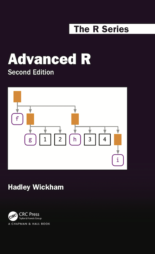
geom_histogram
same number of observations with different sd will give a different number of bins in each facet.
sd <- c(1, 5, 15)
n <- 100

df <- data.frame(x = rnorm(3 * n, sd = sd), sd = rep(sd, n))

head(df)
## x sd
## 1 0.8702774 1
## 2 4.2134232 5
## 3 -9.6693749 15
## 4 -0.5572895 1
## 5 -2.0192570 5
## 6 10.4718642 15ggplot(df, aes(x)) +
geom_histogram(binwidth = 2) +
facet_wrap(~ sd, scales = "free_x") +
labs(x = NULL)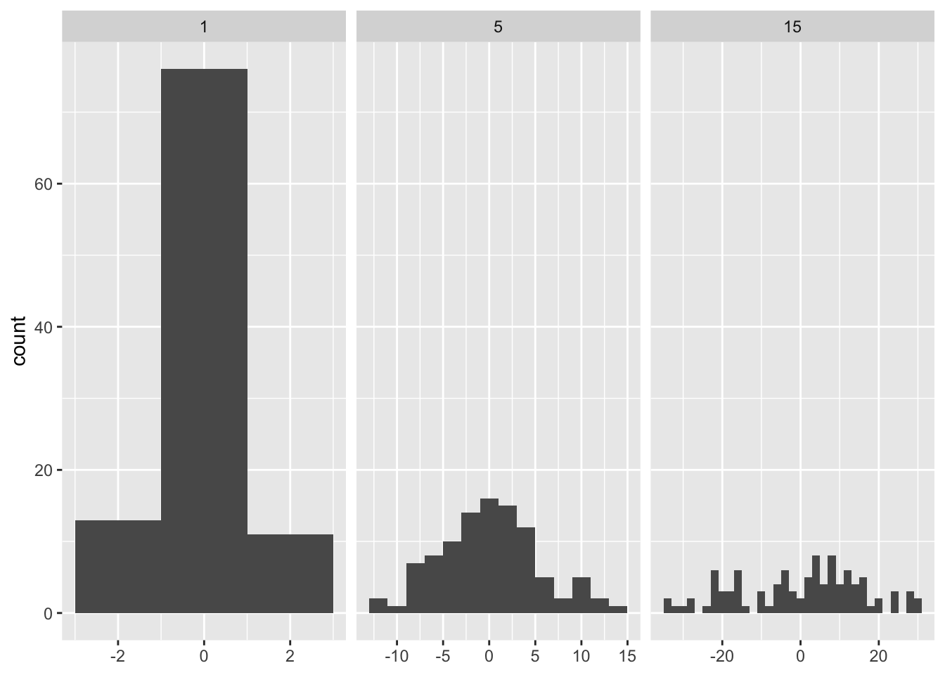
In order to fix the number of bins per facet we can pass a function instead.
binwidth_bins <- function(n) {
  force(n)

  function(x) {
    (max(x) - min(x)) / n
  }
}

ggplot(df, aes(x)) +
  geom_histogram(binwidth = binwidth_bins(20)) +
  facet_wrap(~ sd, scales = "free_x") +
  labs(x = NULL)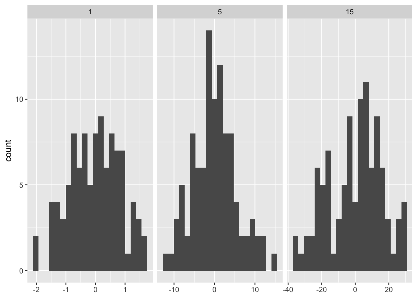
geom_function() and stat_function()
in ggplot2 stat_function() and geom_function() allow you to plot a function that returns y of a given x values.
Here the density derived from 100 samples from a normal distribution vs the actual normal density function.
ggplot(data.frame(x = rnorm(100)), aes(x)) +
  geom_density() +
  geom_function(fun = dnorm, colour = "red")
or using statfunction()
ggplot(data.frame(x = rnorm(100)), aes(x)) +
  geom_density() +
  stat_function(fun = dnorm, geom = "line", colour = "red")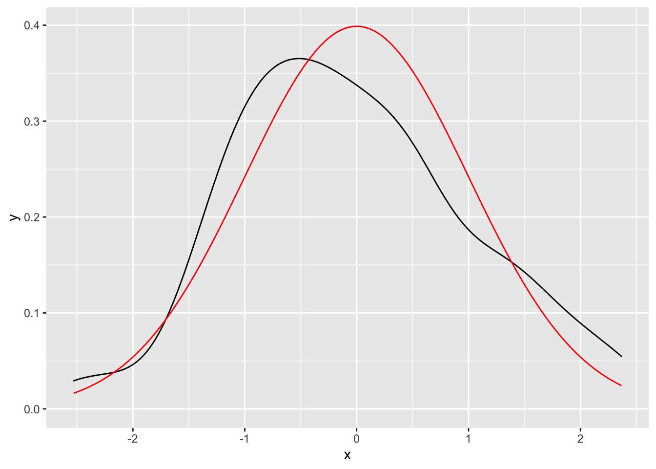
function only
ggplot() +
  stat_function(fun = dnorm, geom = "line", colour = "red") +
  lims(x = c(-3, +3))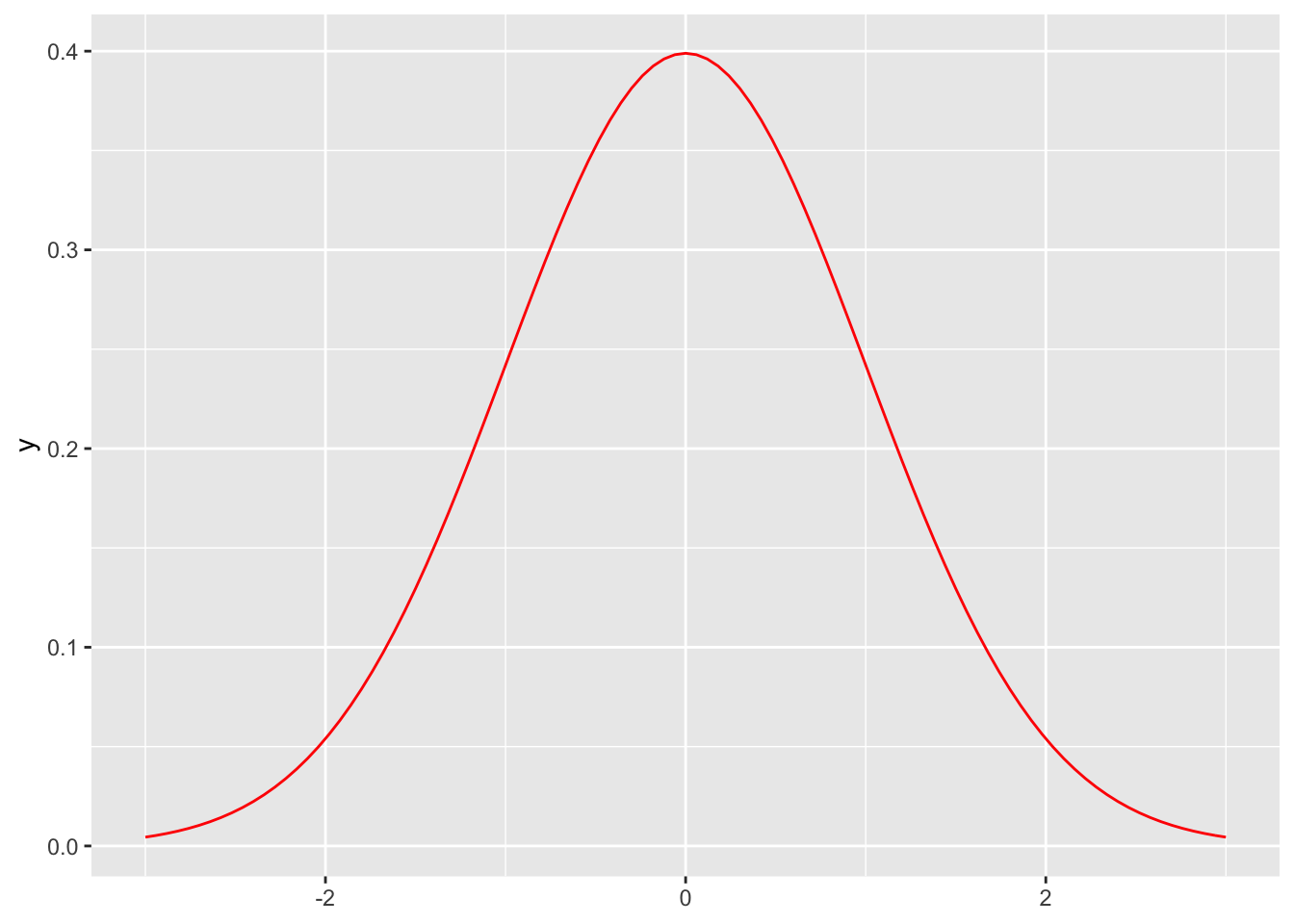
Boxcox Transformation
boxcox transformation is a power transformation that is used to convert non normal distributed values to a normal distribution. The degree of the transformation is defined by an unspecified lambda. For lambda == 0 it results in a log(x) transformation.
boxcox1 <- function(x, lambda) {
  if (lambda == 0) {
    log(x)
  } else {
    (x ^ lambda - 1) / lambda
  }
}
in order to plot boxcox transformations for different lambdas we need to generate a function that takes only one x argument.
boxcox2 <- function(lambda) {
  if (lambda == 0) {
    function(x) log(x)
  } else {
    function(x) (x ^ lambda - 1) / lambda
  }
}

ggplot() +
  geom_function(aes(colour = 0), fun = boxcox2(0)) +
  geom_function(aes(colour = 1), fun = boxcox2(1)) +
  geom_function(aes(colour = 1.5), fun = boxcox2(1.5)) +
  lims(x = c(0, 10))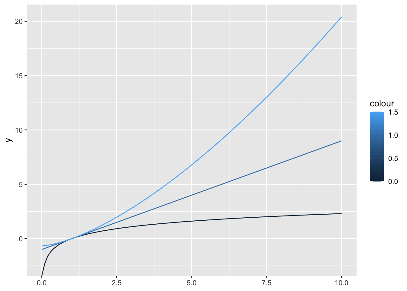
we can wrap the geom calls into another function and use lapply()
geoms_boxcox <- function(lambda, ...) {
  geom_function(aes(colour = lambda), fun = boxcox2(lambda), ...)
}

ggplot() +
  lapply(c(0, 1, 1.5), geoms_boxcox) +
  lims(x = c(0, 10))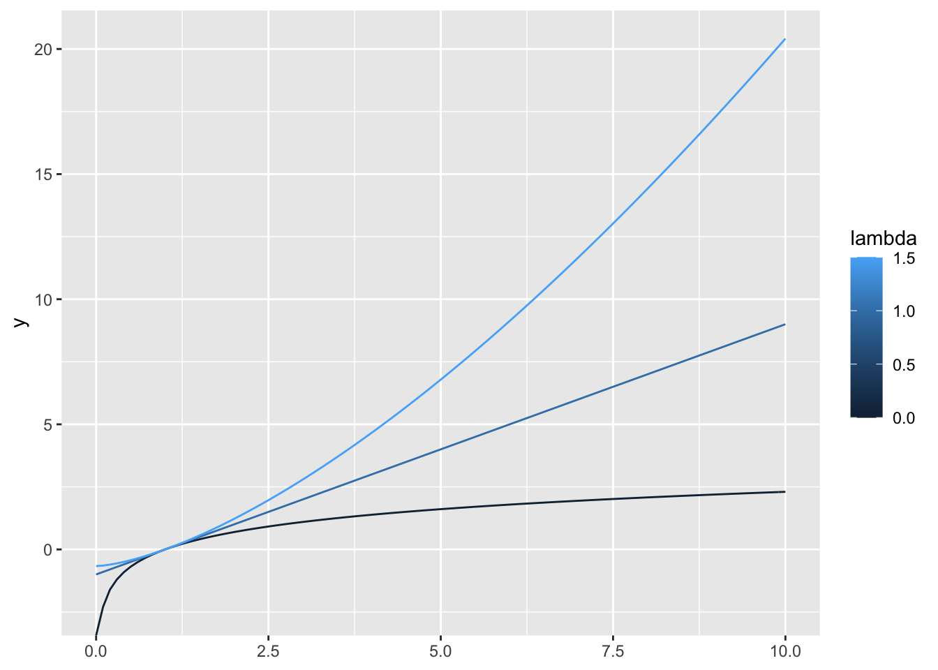
Bootstraping
bootstrap resampling to permute columns in a dataframe
boot_permute <- function(df, var) {
  n <- nrow(df)
  force(var)

  function() {
    col <- df[[var]]
    col[sample(n, replace = TRUE)]
  }
}

boot_mtcars1 <- boot_permute(mtcars, "mpg")
head(boot_mtcars1())
## [1] 32.4 32.4 24.4 33.9 21.4 21.5head(boot_mtcars1())## [1] 26.0 13.3 15.0 17.3 15.2 15.5Imagine we would want to resample residuals of a model in order to bootstrap error statistics
mod <- lm(mpg ~ wt + disp, data = mtcars)
# fitted returns fitted values, same as predict without newdata argument
fitted <- unname(fitted(mod))
pred <- unname(predict(mod))
stopifnot(identical(round(fitted, 6), round(pred, 6)))

resid <- unname(resid(mod))
head(resid)
## [1] -2.345433 -1.490972 -2.472367 1.785333 1.647193 -1.278631boot_resid <- boot_permute(tibble(resid = resid), "resid")
head(boot_resid())## [1] -2.472367 -3.408680 6.348440 2.192792 -2.862147 -2.317052head(boot_resid())## [1] 1.3973583 -2.1005656 0.8901898 -0.2734911 -2.4723669 -2.0291802we can refactor, and remove the model fitting into the factory.
boot_model <- function(df, formula) {
  mod <- lm(formula, data = df)
  resid <- unname(resid(mod))
  # remove the model to save memory
  rm(mod)

  function() {
    sample(resid, size = length(resid), replace = TRUE)
  }
}

boot_mtcars2 <- boot_model(mtcars, mpg ~ wt + disp)
head(boot_mtcars2())
## [1] 2.728799 2.192792 2.728799 6.348440 -2.317200 -1.278631head(boot_mtcars2())## [1] -2.47236688 -0.03421046 0.89018976 2.19486787 -2.31719966 0.22354778Maximum Likelihod Estimation
find the parameter of a distribution that fits some observed values
lprob_poisson <- function(lambda, x) {
  n <- length(x)
  (log(lambda) * sum(x)) - (n * lambda) - sum(lfactorial(x))
}

obs <- c(41, 30, 31, 38, 29, 24, 30, 29, 31, 38)

lprob_poisson(10, obs)
## [1] -183.6405lprob_poisson(20, obs)## [1] -61.14028lprob_poisson(30, obs)## [1] -30.98598the term sum(lfactorial(x) is independent of lambda and can be precomputed to optimise the calculation
c <- sum(lfactorial(x))

lprob_poisson1 <- function(lambda, x, c) {
  n <- length(x)
  (log(lambda) * sum(x)) - (n * lambda) - c
}

lprob_poisson(10, obs)
## [1] -183.6405we can also move x and c into the function
lprob_poisson2 <- function(x) {

  # we do not need to force(x)
  # since it is not used by the
  # returned function
  n <-length(x)
  c <- sum(lfactorial(x))
  sum_x <- sum(x)

  function(lambda) {
    (log(lambda) * sum_x) - (n * lambda) - c
  }
}

ll1 <- lprob_poisson2(obs)
ll1(10)
## [1] -183.6405we can use optimise to find the best value
optimise(f = ll1, interval = c(0, 100), maximum = TRUE)## $maximum
## [1] 32.09999
##
## $objective
## [1] -30.26755Function Operators
Functions that take a function as an argument and return a modfified function. Are called decorators in python.
purrr::safely()and friendsmemoise::memoise()(see below)- any reusable wrapper, for example one that automatically retries a give function on failure
memoise::memoise()
caching the results of a slow function when executed again with the same arguments
slow_function <- function(x) {
  Sys.sleep(1)
  x * 10 * runif(1)
}

# different results
system.time(print(slow_function(1)))
## [1] 3.095154## user system elapsed
## 0.001 0.000 1.004system.time(print(slow_function(1)))## [1] 9.585923## user system elapsed
## 0.004 0.000 1.008fast_function <- memoise::memoise(slow_function)
# same results because cached result is returned
system.time(print(fast_function(1)))## [1] 1.817053## user system elapsed
## 0.001 0.000 1.003system.time(print(fast_function(1)))## [1] 1.817053## user system elapsed
## 0.022 0.000 0.022# different result because argument has changed
system.time(print(fast_function(2)))## [1] 6.450071## user system elapsed
## 0 0 1Recursion
a classical example for recursive functions is the fibinacci sequence
fib <- function(n) {
  if (n < 2) return(1)
  fib(n - 2) + fib(n - 1)
}
system.time(print(fib(23)))
## [1] 46368## user system elapsed
## 0.050 0.002 0.052system.time(print(fib(33)))## [1] 5702887## user system elapsed
## 5.056 0.050 5.138memoise::memoise() will cache the results
fib2 <- memoise::memoise(function(n) {
  if (n < 2) return(1)
  fib2(n - 2) + fib2(n - 1)
})

system.time(fib2(23))
## user system elapsed
## 0.009 0.000 0.010system.time(fib2(33))## user system elapsed
## 0.003 0.000 0.003OOP
- encapsulated OOP
object.method(arg1, arg2)
- functional OOP
generic(object, arg1, arg2)
S3
Functional OOP framework that is most commonly used in R.
There are very few constrictions for creating S3 classes but some conventions.
- create a low-level constructor that creates objects with the right structure called
new_myclass()
- a validator that performs computationally expensive checks, called
validate_myclass()
- a user-friendly helper called
myclass()
simaerep example
the simaerep v0.3.1 package currently performs a sequence of operations on a dataframe. Each operations requires a different function that takes a data.frame and returns a modified version. We could simplify the interface for the users by grouping all those operations using S3 classes.
There is no function wrapping the entire workflow because we want intermediary results to be accessible and visible. By convention a function returns only one object which would then only return the final dataframe df_eval. Then we would loose df_site and df_sim_sites for plotting and inspection.
Advantages:
- simplified user interface
- input checks only need to run once
- preserve intermediary results as class attributes
# devtools::install_github("openpharma/simaerep@v0.3.1")

suppressPackageStartupMessages(library("simaerep"))

set.seed(1)

df_visit <- sim_test_data_study(
  n_pat = 1000, # number of patients in study
  n_sites = 100, # number of sites in study
  frac_site_with_ur = 0.05, # fraction of sites under-reporting
  ur_rate = 0.4, # rate of under-reporting
  ae_per_visit_mean = 0.5 # mean AE per patient visit
)

df_visit$study_id <- "A"

df_site <- site_aggr(df_visit)

df_sim_sites <- sim_sites(df_site, df_visit, r = 1000)

df_eval <- eval_sites(df_sim_sites)

plot_study(df_visit, df_site, df_eval, study = "A") 
constructor
new_simaerep <- function(df_site,
                           df_sim_sites,
                           df_eval,
                           r) {

  structure(
    list(
      df_site = df_site,
      df_sim_sites = df_sim_sites,
      df_eval = df_eval,
      r = r
    ),
    class = "simaerep"
  )
}
validator
validate_simaerep <- function(obj) {
  comp <- sort(attributes(obj)$names) ==  sort(c("df_site", "df_sim_sites", "df_eval", "r"))
  stopifnot(all(comp))
  return(obj)
}
user-friendly constructor
simaerep <- function(df_visit, r = 1000) {

  df_site <- site_aggr(df_visit)

  df_sim_sites <- sim_sites(df_site, df_visit, r = 1000)

  df_eval <- eval_sites(df_sim_sites)

  validate_simaerep(
    new_simaerep(
      df_site,
      df_sim_sites,
      df_eval,
      r
    )
  )
}

simaerep_studyA <- simaerep(df_visit)

str(simaerep_studyA)
## List of 4
## $ df_site : tibble [100 × 6] (S3: tbl_df/tbl/data.frame)
## ..$ study_id : chr [1:100] "A" "A" "A" "A" ...
## ..$ site_number : chr [1:100] "S0001" "S0002" "S0003" "S0004" ...
## ..$ n_pat : int [1:100] 10 10 10 10 10 10 10 10 10 10 ...
## ..$ n_pat_with_med75 : int [1:100] 9 8 9 9 7 8 10 7 10 8 ...
## ..$ visit_med75 : Named num [1:100] 15 19 14 16 18 19 17 16 16 16 ...
## .. ..- attr(*, "names")= chr [1:100] "80%" "80%" "80%" "80%" ...
## ..$ mean_ae_site_med75: num [1:100] 4 5.12 4.22 4.67 6.29 ...
## $ df_sim_sites: tibble [100 × 9] (S3: tbl_df/tbl/data.frame)
## ..$ study_id : chr [1:100] "A" "A" "A" "A" ...
## ..$ site_number : chr [1:100] "S0001" "S0002" "S0003" "S0004" ...
## ..$ n_pat : int [1:100] 10 10 10 10 10 10 10 10 10 10 ...
## ..$ n_pat_with_med75 : int [1:100] 9 8 9 9 7 8 10 7 10 8 ...
## ..$ visit_med75 : Named num [1:100] 15 19 14 16 18 19 17 16 16 16 ...
## .. ..- attr(*, "names")= chr [1:100] "80%" "80%" "80%" "80%" ...
## ..$ mean_ae_site_med75 : num [1:100] 4 5.12 4.22 4.67 6.29 ...
## ..$ mean_ae_study_med75: num [1:100] 7.38 9.33 6.92 7.91 8.84 ...
## ..$ pval : num [1:100] 7.14e-05 3.15e-05 1.38e-03 2.60e-04 2.11e-02 ...
## ..$ prob_low : num [1:100] 0 0 0 0 0.012 0.431 0.04 1 1 0.395 ...
## $ df_eval : tibble [100 × 13] (S3: tbl_df/tbl/data.frame)
## ..$ study_id : chr [1:100] "A" "A" "A" "A" ...
## ..$ site_number : chr [1:100] "S0002" "S0001" "S0004" "S0003" ...
## ..$ n_pat : int [1:100] 10 10 10 10 10 10 10 10 10 10 ...
## ..$ n_pat_with_med75 : int [1:100] 8 9 9 9 10 7 9 9 9 10 ...
## ..$ visit_med75 : Named num [1:100] 19 15 16 14 15 18 17 15 16 17 ...
## .. ..- attr(*, "names")= chr [1:100] "80%" "80%" "80%" "80%" ...
## ..$ mean_ae_site_med75 : num [1:100] 5.12 4 4.67 4.22 5.4 ...
## ..$ mean_ae_study_med75: num [1:100] 9.33 7.38 7.91 6.92 7.37 ...
## ..$ pval : num [1:100] 3.15e-05 7.14e-05 2.60e-04 1.38e-03 2.19e-02 ...
## ..$ prob_low : num [1:100] 0 0 0 0 0.009 0.012 0.017 0.036 0.038 0.04 ...
## ..$ pval_adj : num [1:100] 0.00315 0.00357 0.00867 0.03444 0.36483 ...
## ..$ pval_prob_ur : num [1:100] 0.997 0.996 0.991 0.966 0.635 ...
## ..$ prob_low_adj : num [1:100] 0 0 0 0 0.18 ...
## ..$ prob_low_prob_ur : num [1:100] 1 1 1 1 0.82 ...
## $ r : num 1000
## - attr(*, "class")= chr "simaerep"adding some class methods for common generic functions like print(), plot()
print.simaerep <- function(obj) {
  studies <- unique(obj$df_site$study_id)
  print(paste("AE underreporting for studies:", studies))
}

print(simaerep_studyA)
## [1] "AE underreporting for studies: A"plot.simaerep <- function(obj, df_visit, study, what = c("study", "med75")) {
stopifnot(study %in% unique(df_visit$study_id))
what <- match.arg(what)
.f <- switch(
what,
study = function(...) simaerep::plot_study(..., df_eval = obj$df_eval, study = study),
med75 = function(...) simaerep::plot_visit_med75(..., study_id_str = study)
)
.f(df_visit = df_visit, df_site = obj$df_site)
}
plot(simaerep_studyA, df_visit, study = "A", what = "study")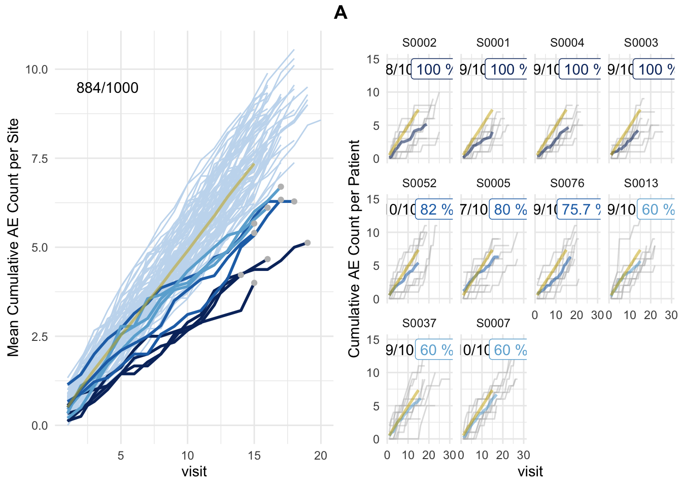
plot(simaerep_studyA, df_visit, study = "A", what = "med75")## purple line: mean site ae of patients with visit_med75
## grey line: patient included
## black dashed line: patient excluded
## dotted vertical line: visit_med75, 0.75 x median of maximum patient visits of site
## solid vertical line: visit_med75 adjusted, increased to minimum maximum patient visit of included patients
## dashed vertical line: maximum value for visit_med75 adjusted, 80% quantile of maximum patient visits of study
to this point we have not:
- created new generic functions
- used class inheritance
A class that inherits from another class mus carry all its parents attributes, we can implement this by modifying the parent constructor as below and by calling the parent constructor from within the child constructor.
Here we will create two classes one for initiating a simaerep object and the initial df_site aggregation step and one for the simulation.
new_simaerep <- function(df_site, ..., class = character()) {
  structure(
    list(
      df_site = df_site,
      ...
    ),
    class = c(class, "simaerep")
  )
}

validate_simaerep <- function(obj) {
  comp <- attributes(obj)$names ==  "df_site"
  stopifnot(all(comp))
  return(obj)
}

simaerep <- function(df_visit) {

  df_site <- site_aggr(df_visit)

  validate_simaerep(
    new_simaerep(
      df_site
    )
  )
}

simaerep_studyA <- simaerep(df_visit)

str(simaerep_studyA)
## List of 1
## $ df_site: tibble [100 × 6] (S3: tbl_df/tbl/data.frame)
## ..$ study_id : chr [1:100] "A" "A" "A" "A" ...
## ..$ site_number : chr [1:100] "S0001" "S0002" "S0003" "S0004" ...
## ..$ n_pat : int [1:100] 10 10 10 10 10 10 10 10 10 10 ...
## ..$ n_pat_with_med75 : int [1:100] 9 8 9 9 7 8 10 7 10 8 ...
## ..$ visit_med75 : Named num [1:100] 15 19 14 16 18 19 17 16 16 16 ...
## .. ..- attr(*, "names")= chr [1:100] "80%" "80%" "80%" "80%" ...
## ..$ mean_ae_site_med75: num [1:100] 4 5.12 4.22 4.67 6.29 ...
## - attr(*, "class")= chr "simaerep"new_simaerep_sim <- function(df_site, df_sim_sites, df_eval, r) {
new_simaerep(
df_site = df_site,
df_sim_sites = df_sim_sites,
df_eval = df_eval,
r = r,
class = "simaerep_sim"
)
}
validate_simaerep_sim <- function(obj) {
comp <- sort(attributes(obj)$names) == sort(c("df_site", "df_sim_sites", "df_eval", "r"))
stopifnot(all(comp))
return(obj)
}next we define a new generic method called sim that starts the simulation which returns the new class simaerep_sim. The process that finds the right method to call for an object called with a generic function is called method dispatching.
# define generic function
sim <- function(obj, ...) {
  UseMethod("sim")
}

sim.simaerep <- function(obj, df_visit, r = 1000) {

  df_sim_sites <- sim_sites(obj$df_site, df_visit, r = r)

  df_eval <- eval_sites(df_sim_sites)

  validate_simaerep_sim(
    new_simaerep_sim(
      df_site,
      df_sim_sites,
      df_eval,
      r
    )
  )
}

simaerep_studyA_sim <- sim(simaerep_studyA, df_visit)

str(simaerep_studyA_sim)
## List of 4
## $ df_site : tibble [100 × 6] (S3: tbl_df/tbl/data.frame)
## ..$ study_id : chr [1:100] "A" "A" "A" "A" ...
## ..$ site_number : chr [1:100] "S0001" "S0002" "S0003" "S0004" ...
## ..$ n_pat : int [1:100] 10 10 10 10 10 10 10 10 10 10 ...
## ..$ n_pat_with_med75 : int [1:100] 9 8 9 9 7 8 10 7 10 8 ...
## ..$ visit_med75 : Named num [1:100] 15 19 14 16 18 19 17 16 16 16 ...
## .. ..- attr(*, "names")= chr [1:100] "80%" "80%" "80%" "80%" ...
## ..$ mean_ae_site_med75: num [1:100] 4 5.12 4.22 4.67 6.29 ...
## $ df_sim_sites: tibble [100 × 9] (S3: tbl_df/tbl/data.frame)
## ..$ study_id : chr [1:100] "A" "A" "A" "A" ...
## ..$ site_number : chr [1:100] "S0001" "S0002" "S0003" "S0004" ...
## ..$ n_pat : int [1:100] 10 10 10 10 10 10 10 10 10 10 ...
## ..$ n_pat_with_med75 : int [1:100] 9 8 9 9 7 8 10 7 10 8 ...
## ..$ visit_med75 : Named num [1:100] 15 19 14 16 18 19 17 16 16 16 ...
## .. ..- attr(*, "names")= chr [1:100] "80%" "80%" "80%" "80%" ...
## ..$ mean_ae_site_med75 : num [1:100] 4 5.12 4.22 4.67 6.29 ...
## ..$ mean_ae_study_med75: num [1:100] 7.38 9.33 6.92 7.91 8.84 ...
## ..$ pval : num [1:100] 7.14e-05 3.15e-05 1.38e-03 2.60e-04 2.11e-02 ...
## ..$ prob_low : num [1:100] 0 0 0 0 0.012 0.431 0.04 1 1 0.395 ...
## $ df_eval : tibble [100 × 13] (S3: tbl_df/tbl/data.frame)
## ..$ study_id : chr [1:100] "A" "A" "A" "A" ...
## ..$ site_number : chr [1:100] "S0002" "S0001" "S0004" "S0003" ...
## ..$ n_pat : int [1:100] 10 10 10 10 10 10 10 10 10 10 ...
## ..$ n_pat_with_med75 : int [1:100] 8 9 9 9 10 7 9 9 9 10 ...
## ..$ visit_med75 : Named num [1:100] 19 15 16 14 15 18 17 15 16 17 ...
## .. ..- attr(*, "names")= chr [1:100] "80%" "80%" "80%" "80%" ...
## ..$ mean_ae_site_med75 : num [1:100] 5.12 4 4.67 4.22 5.4 ...
## ..$ mean_ae_study_med75: num [1:100] 9.33 7.38 7.91 6.92 7.37 ...
## ..$ pval : num [1:100] 3.15e-05 7.14e-05 2.60e-04 1.38e-03 2.19e-02 ...
## ..$ prob_low : num [1:100] 0 0 0 0 0.009 0.012 0.017 0.036 0.038 0.04 ...
## ..$ pval_adj : num [1:100] 0.00315 0.00357 0.00867 0.03444 0.36483 ...
## ..$ pval_prob_ur : num [1:100] 0.997 0.996 0.991 0.966 0.635 ...
## ..$ prob_low_adj : num [1:100] 0 0 0 0 0.18 ...
## ..$ prob_low_prob_ur : num [1:100] 1 1 1 1 0.82 ...
## $ r : num 1000
## - attr(*, "class")= chr [1:2] "simaerep_sim" "simaerep"class(simaerep_studyA_sim)## [1] "simaerep_sim" "simaerep"plot.simaerep <- function(obj, df_visit, study,
... # we need ... to ignore additional arguments when called with NextMethod()
) {
simaerep::plot_visit_med75(df_visit, obj$df_site, study_id_str = study)
}override plot method of parent class, and use user-supplied argument to switch back to parent class method using NextMethod()
plot.simaerep_sim <- function(obj, df_visit, study, what = c("study", "med75")) {
  what <- match.arg(what)
  if (what == "study") {
    simaerep::plot_study(df_visit, obj$df_site, obj$df_eval, study = study)
  } else {
    # calls parent class method using all original arguments
    NextMethod()
  }
}


plot(simaerep_studyA_sim, df_visit, study = "A", what = "study")
plot(simaerep_studyA_sim, df_visit, study = "A", what = "med75")## purple line: mean site ae of patients with visit_med75
## grey line: patient included
## black dashed line: patient excluded
## dotted vertical line: visit_med75, 0.75 x median of maximum patient visits of site
## solid vertical line: visit_med75 adjusted, increased to minimum maximum patient visit of included patients
## dashed vertical line: maximum value for visit_med75 adjusted, 80% quantile of maximum patient visits of study
plot(simaerep_studyA_sim, df_visit, study = "A", what = "XXX")## Error in match.arg(what): 'arg' should be one of "study", "med75"plot(simaerep_studyA, df_visit, study = "A")## purple line: mean site ae of patients with visit_med75
## grey line: patient included
## black dashed line: patient excluded
## dotted vertical line: visit_med75, 0.75 x median of maximum patient visits of site
## solid vertical line: visit_med75 adjusted, increased to minimum maximum patient visit of included patients
## dashed vertical line: maximum value for visit_med75 adjusted, 80% quantile of maximum patient visits of study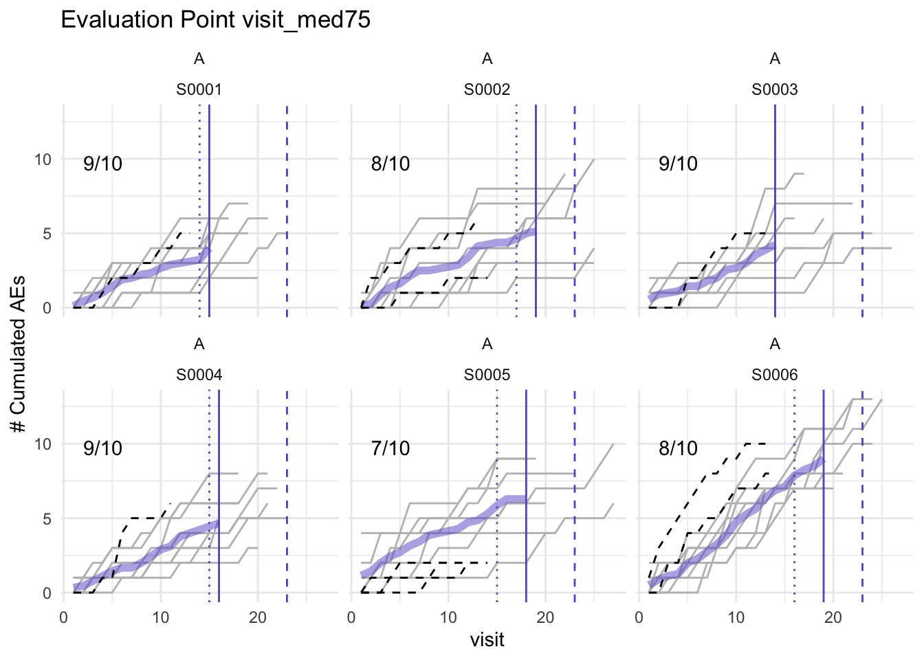
sloop provides some function to investigate S3 class behavior.
sloop::s3_methods_class("simaerep")## # A tibble: 3 × 4
## generic class visible source
## <chr> <chr> <lgl> <chr>
## 1 plot simaerep TRUE .GlobalEnv
## 2 print simaerep TRUE .GlobalEnv
## 3 sim simaerep TRUE .GlobalEnvsloop::s3_methods_class("simaerep_sim")## # A tibble: 1 × 4
## generic class visible source
## <chr> <chr> <lgl> <chr>
## 1 plot simaerep_sim TRUE .GlobalEnvsloop::s3_methods_generic("sim")## # A tibble: 1 × 4
## generic class visible source
## <chr> <chr> <lgl> <chr>
## 1 sim simaerep TRUE .GlobalEnvsloop::s3_dispatch(plot(simaerep_studyA_sim, df_visit, study = "A"))## => plot.simaerep_sim
## -> plot.simaerep
## * plot.defaultsloop::s3_dispatch(plot(simaerep_studyA, df_visit, study = "A"))## => plot.simaerep
## * plot.defaultR6
R6 uses the encapsulated OOP framework, commonly used in shiny. Works like object in python.
- Use
R6::R6Class()to construct classes - Pass a list with attributes (static values) and methods (functions)
- Within methods refer to the class as
selfand subset with$(self$attribute,self.method()) - Instantiate objects by calling
x <- Class$new() - methods can be chained
x$add(1)$sub(1) initialize()method overrisenew()and works like__init()in python- inherit by using the
inheritargument ofR6::R6Class() - pass private and public attributes and classes using the
privatandpublicarguments ofR6::R6Class() - active fields look like attributes but are methods, can run additional checks
- instantiated R6 classes behave like python objects modifying one object will also modify all of its copies
- always put randomized default values that you do not want to share across instances into the initialize function
S4
Mostly used for bioconductor packages uses functional OOP framework. A well-known package that uses S4 is ROCR and lubridate
- much stricter framework than S3
- makes use of specialized functions like
setClass(),setGeneric(),setMethod() - all functions are distributed with R in the
methodspackage (which should be explicitly loaded so show S4 framework is used and to avoid problems when running non-interactive mode) - attributes are slots which can be subset using
@ - supports multiple inheritance and multiple dispatch (which should be avoided because its complicated)
Slots
- when instantiated objects slot’s are automatically checked if they contain the correct data types
setValidity(),validObject()can be used to extend checks and to validate existing objects
Conventions
- CamelCase
- provide constructor with same name as class
- write generics that call and set slot values
Multiple Inheritence
in case a class inherits from multiple classes the method that is closest to the class is chosen. If two methods are matching the method for the class which has a higher lexical order is chosen.
Multiple dispatch
If a generic uses two classes as input both classes are searched for methods.
S4 vs S3
- S4 more suitable for larger teams
- S4 is better with many inter related objects (for example provide methods via generics for combinations of different types of sparse matrices)