Six Sigma with R - Notes

Six Sigma with R. Statistical Engineering for Process Improvement (Cano EL, Moguerza JM and Redchuk A, 2012).
R packages
suppressPackageStartupMessages(library(tidyverse))
library(SixSigma)
library(DiagrammeR)
library(nomnoml)
6 Sigma
6 sigma is framework for process improvement and is not limited to process control. It consists of a cycle of several stages all of which are employing the scientific method:
DMAIC cycle:
- Define
- Measure
- Analyse
- Improve
- Control
Define
Process Charts
High Level:
- Process fits onto one power point slide
- Onboarding new people
- SIPOC, VSM are commonly used in six sigma
six sigma focuses on the inputs and the output of a process.
Inputs are the 6 Ms:
- Manpower
- Materials
- Machines
- Methods
- Measurements
- Mother Nature (Environment)
Output:
- CTQ (Crtitical to Quality Characteristics)
- key measurable characteristics of a product or process whose performance standards or specification limits must be met
For example the processing of Individual Case Safety Reports for submission to the Health Authorities.
nomnoml::nomnoml(
"#direction: right
#padding: 20
#spacing: 100

[Input 6M's|ICSR; IT System; Legislation; Process Owner; PV Associate]

[Input 6M's]->[Output CTQs|Recipients; Submission Status; Processing Time; Compliance Status; Medical Risk; Compliance Risk]"
)
Low Level:
- more elaborate flow charts
- UML activity diagram provides some standards.
- BMPN Swim Lanes
UML/BMPN process maps do not focus on 6 Ms and CTQs. We can continue the simplified input output diagram ba adding more steps to the process. The input for each individual consists of elements of the initial 6M input (X) or the output produced by one of the previous steps. Each Step can have parameters (x) that influence the quality of the output. Each step output has quality features (y). Which can be included in the final output CTQs (Y).
nomnoml::nomnoml(
"#title: ICSR Processing
#direction: right
#padding: 20
#spacing: 100


[Input 6M's (X)|ICSR; IT System; Legislation; Process Owner; PV Associate; Product]
[Input 6M's (X)]->[<table> Ensure Completeness|
    Input| ICSR; IT System; PV Associate||
    Substeps/Methods| follow_up()||
    Parameters(x); influence Quality|ICSR Source||
    Quality Features(y)|ICSR Completeness; Time
]
[Ensure Completeness]->[Medical Review|
  ICSR Complete; IT System; PV Associate|
  review(); follow_up()|
  ICSR Complexity;Source Accessibility; Privacy Laws|
  Medical Risk; Causality;Severity; Labelling; Product Approval; Time
]
[Medical Review]->[Apply Submission Legislation|
  ICSR Reviewed; Legislation; IT System; Process Owner|
  encode_legislation(); qc_submission_status(); submit()|
  Legislation Complexity; Number Cases to Review|
  Compliance Risk; Submission Status; Recipients; Time; QC Status
]
[Apply Submission Legislation]->[Output CTQs (Y)|
    Recipients; Submission Status; Processing Time; Compliance Status; Medical Risk; Compliance Risk; QC Status
]")
Analyse
Loss Function Analysis
Loss functioncan be used during the DMAIC measure phase by calculating expected loss as a product of average loss per item by number of items. It can also be used to set the upper and lower specification limits (USL/LSL).
In six sigma loss increases quadratically when deviating from the process target not only after crossing a threshold.
Loss = k(Y-Y0)^2
df <- SixSigma::ss.data.bolts
head(df)
## diameter
## 1 10.4042
## 2 10.2584
## 3 9.9478
## 4 10.2678
## 5 10.1144
## 6 9.9830lfa <- SixSigma::ss.lfa(
lfa.data = df,
lfa.ctq = "diameter",
lfa.Delta = 0.5, #process tolerance,
lfa.Y0 = 10, #process target
lfa.L0 = 0.001, #cost at tolerance limit
lfa.size = 1e5
)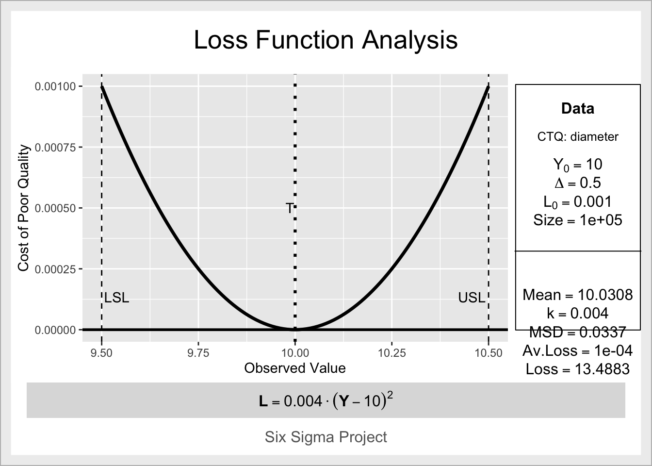
lfa## $lfa.k
## [1] 0.004
##
## $lfa.lf
## expression(bold(L == 0.004 %.% (Y - 10)^2))
##
## $lfa.MSD
## [1] 0.03372065
##
## $lfa.avLoss
## [1] 0.0001348826
##
## $lfa.Loss
## [1] 13.48826loss_at_10.25 <- lfa$lfa.k * (10.25 - 10)^2
loss_at_10.25## [1] 0.00025Measurement System Analysis
Measurement system analysis (MSA) is also known as gage R&R study identifies and quantifies the sources of variation that influence the measurement system.
In a good measurement the only variability is random and stems from the difference in the parts that are measured and not from the so called appraisers (operator, measurement machines, time of the day). MSA uses ANOVA to compare the ratio of between-groups variability to within-groups variability. If this ratio is large, we conclude that the groups are significantly different.
- G R&R (appraisal) contribution to variation must be low and is the sum of Repeatability (appraisers) and Reproducibility (interactions)
- part to part contribution to variation must be high
- total variation = R&R + part to part
df <- SixSigma::ss.data.rr
head(df)
## prototype operator run time1 time2
## 1 prot #1 op #1 run #1 1.27 1.15
## 2 prot #1 op #1 run #2 0.90 1.31
## 3 prot #1 op #1 run #3 1.09 1.25
## 4 prot #2 op #1 run #1 1.12 1.36
## 5 prot #2 op #1 run #2 1.09 1.41
## 6 prot #2 op #1 run #3 1.15 1.37rr <- SixSigma::ss.rr(
var = time1,
part = prototype,
appr = operator,
data = df,
alphaLim = 0.05,
errorTerm = "Interaction",
lsl = 0.7,
usl = 1.8,
method = "crossed" #crossed uses all possible combinations of parts and appraisals
# https://blog.minitab.com/en/a-simple-guide-to-gage-randr-for-destructive-testing
)## Complete model (with interaction):
##
## Df Sum Sq Mean Sq F value Pr(>F)
## prototype 2 1.2007 0.6004 28.040 2.95e-06
## operator 2 0.0529 0.0265 1.236 0.314
## prototype:operator 4 0.0834 0.0208 0.974 0.446
## Repeatability 18 0.3854 0.0214
## Total 26 1.7225
##
## alpha for removing interaction: 0.05
##
##
## Reduced model (without interaction):
##
## Df Sum Sq Mean Sq F value Pr(>F)
## prototype 2 1.2007 0.6004 28.174 8.56e-07
## operator 2 0.0529 0.0265 1.242 0.308
## Repeatability 22 0.4688 0.0213
## Total 26 1.7225
##
## Gage R&R
##
## VarComp %Contrib
## Total Gage R&R 0.0218822671 25.38
## Repeatability 0.0213087542 24.71
## Reproducibility 0.0005735129 0.67
## operator 0.0005735129 0.67
## Part-To-Part 0.0643389450 74.62
## Total Variation 0.0862212121 100.00
##
## VarComp StdDev StudyVar %StudyVar %Tolerance
## Total Gage R&R 0.0218822671 0.14792656 0.8875594 50.38 80.69
## Repeatability 0.0213087542 0.14597518 0.8758511 49.71 79.62
## Reproducibility 0.0005735129 0.02394813 0.1436888 8.16 13.06
## operator 0.0005735129 0.02394813 0.1436888 8.16 13.06
## Part-To-Part 0.0643389450 0.25365123 1.5219074 86.38 138.36
## Total Variation 0.0862212121 0.29363449 1.7618069 100.00 160.16
##
## Number of Distinct Categories = 2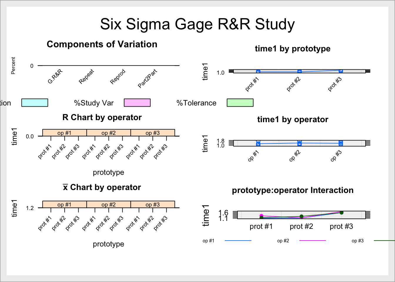
- % Contribution is the total contribution to variability (range)
- % Study Var is the within group variance as percent of the total variance
- % Tolerance should be below 100 for R&R
Capability Analysis
see capability performance indeces from previous blogpost.
ss.study.ca(
  xST = ss.data.ca$Volume, # short-term process data,
  xLT = rnorm(40, 753, 3), # long-term process data
    LSL = 740,
  USL = 760,
  Target = 750,
  alpha = 0.05,
)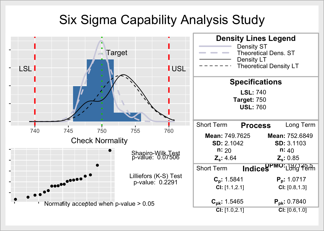
Cpk: min(left right capability index) CI: Confidence Interval of capability index
Improve
Experimental Design
When optimizing a process it is not enough to vary one variable and keep all other variables constant, because we are missing out on interactions. It is best to use a factorial design (binning continuous variables into two) and try all possible combinations in several repeats. Use ANOVA or pairwise t-test to get best result. Include uncontrollable factors in experimental design to find which controllable variables give most robust results when uncontrollable variables vary. Example: Best frozen Pizza recipe for varying baking time and temperature.