Quality Control with R - Notes

Quality Control with R. An ISO Standards Approach (Cano EL, Moguerza JM and Prieto M, 2015).
R packages
qcc seems to be the most popular and best maintained QC package for control charts.
suppressPackageStartupMessages(library(tidyverse))
# we use qcc 3.0 which is not released on CRAN yet
# devtools::install_github("luca-scr/qcc", build = TRUE, build_opts = c("--no-resave-data", "--no-manual"))
library(qcc)
## Package 'qcc' version 3.0
## Type 'citation("qcc")' for citing this R package in publications.library(AcceptanceSampling)
library(SixSigma)
library(DiagrammeR)ISO standard QC Approach
ISO standards are defined by the International Organisation for Standardisation by technical committees using a process that is similar to peer-review. There are a lot of ISO standards covering Quality Control.
QC tools
There are 7 general quality Ishikava tools, each of them is covered by numerous ISO documents.
- Cause and Effect Diagram
- Check sheet
- Control chart
- Histogram
- Pareto Chart
- Scatter Diagram
- Stratification
- Flow charts
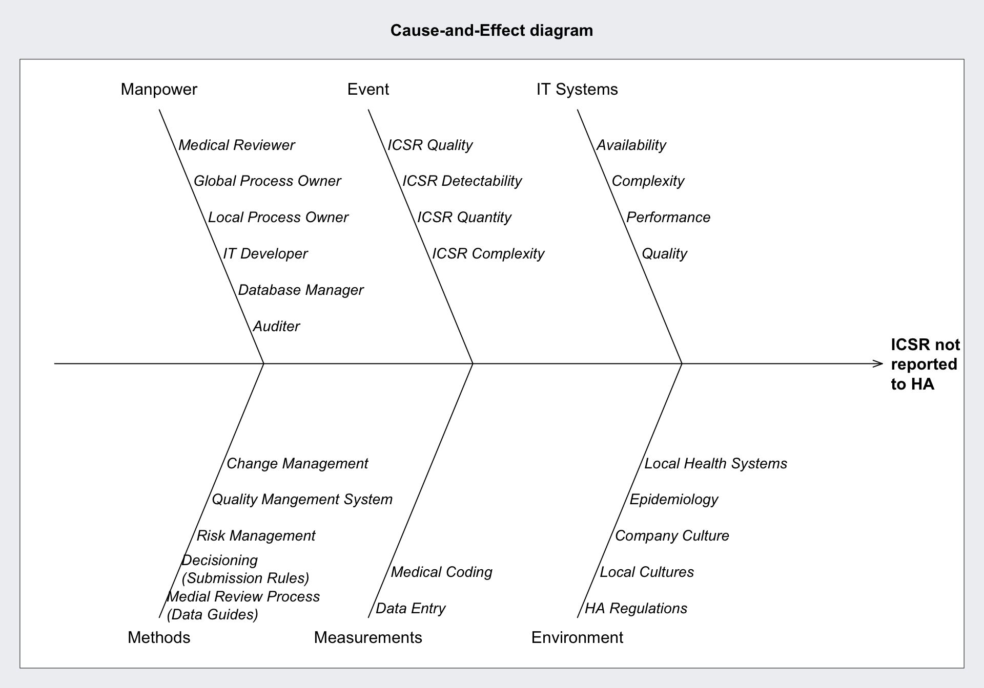
Cause and Effect Diagrams
The effect is usually undesired. As causes for a given effect for processes of the producing industry the ISO standard is 5Ms+E
- Manpower
- Materials
- Machines
- Methods
- Measurements
- Environment
Creatively I would adapt this for data-driven business processes to:
- Manpower
- Events
- IT System
- Methods (Statistics, DevOps, Code base, Manual Processes)
- Measurements of Events (Data Entry, Data Coding)
- Environment (Culture, External Events, Regulations)
Specifically for the reporting of Adverse Drug Reactions in the form of individual case safety reports (ICSR) to Health Authorities (HA).
qcc::causeEffectDiagram(
  cause = list(
    Manpower = c(
      "Medical Reviewer",
      "Global Process Owner",
      "Local Process Owner",
      "IT Developer",
      "Database Manager",
      "Auditer"
    ),
    Event = c(
      "ICSR Quality",
      "ICSR Detectability",
      "ICSR Quantity",
      "ICSR Complexity"
    ),
    `IT Systems` = c(
      "Availability",
      "Complexity",
      "Performance",
      "Quality"
    ),
    Methods = c(
      "Medial Review Process\n(Data Guides)",
      "Decisioning\n(Submission Rules)",
      "Risk Management",
      "Quality Mangement System",
      "Change Management"
    ),
    Measurements = c(
      "Data Entry",
      "Medical Coding"
    ),
    Environment = c(
      "HA Regulations",
      "Local Cultures",
      "Company Culture",
      "Epidemiology",
      "Local Health Systems"
    )
  ),
  effect = "ICSR not\nreported\nto HA"
)
Check Sheets
Serve to generate process related data, should be part of a general data collection plan. Will be automated for most processes.
- Audit Trail Data
- Quality Evidence
- IT Logs
Classically serves to attribute each effect (ICSR not reported to HA) to any of the suspected causes in the cause and effect diagram.
Control Charts (Shewhart Charts)
Process Monitoring Charts, can be used to track whether process KPI are in or out of control.
data("pistonrings")
df <- as_tibble(pistonrings)

df_g1 <- df %>%
  group_by(sample) %>%
  mutate(rwn = row_number()) %>%
  filter(rwn == 1)

qcc_shew <- qcc(
  df$diameter,
  type = "xbar.one",
  rules = c(1, 2, 3, 4)
)

qcc_shew
## ── Quality Control Chart ─────────────────────────
##
## Chart type = xbar.one
## Data (phase I) = df$diameter
## Number of groups = 200
## Group sample size = 1
## Center of group statistics = 74.0036
## Standard deviation = 0.01001461
##
## Control limits at nsigmas = 3
## LCL UCL
## 73.97356 74.03365str(qcc_shew)## List of 12
## $ call : language qcc(data = df$diameter, type = "xbar.one", rules = c(1, 2, 3, 4))
## $ type : chr "xbar.one"
## $ data.name : chr "df$diameter"
## $ data : num [1:200, 1] 74 74 74 74 74 ...
## ..- attr(*, "dimnames")=List of 2
## .. ..$ Group : chr [1:200] "1" "2" "3" "4" ...
## .. ..$ Samples: NULL
## $ statistics: Named num [1:200] 74 74 74 74 74 ...
## ..- attr(*, "names")= chr [1:200] "1" "2" "3" "4" ...
## $ sizes : int [1:200] 1 1 1 1 1 1 1 1 1 1 ...
## $ center : num 74
## $ std.dev : num 0.01
## $ rules : num [1:4] 1 2 3 4
## $ nsigmas : num 3
## $ limits : num [1, 1:2] 74 74
## ..- attr(*, "dimnames")=List of 2
## .. ..$ : chr ""
## .. ..$ : chr [1:2] "LCL" "UCL"
## $ violations: num [1:200] NA NA NA NA NA NA NA NA NA NA ...
## ..- attr(*, "WesternElectricRules")= num [1:4] 1 2 3 4
## - attr(*, "class")= chr "qcc"plot(qcc_shew)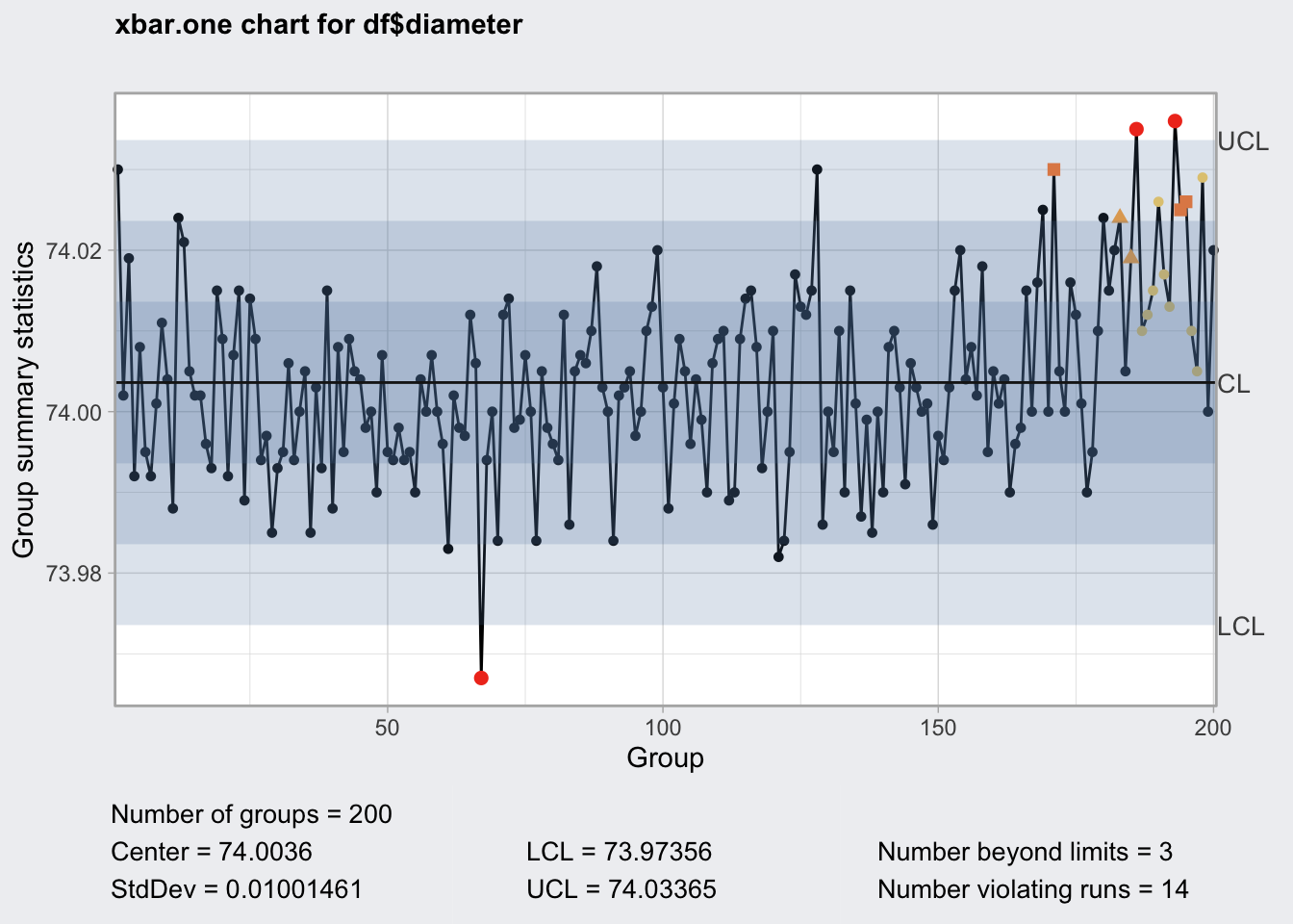
qcc_shew$violations## [1] NA NA NA NA NA NA NA NA NA NA NA NA NA NA NA NA NA NA NA NA NA NA NA NA NA
## [26] NA NA NA NA NA NA NA NA NA NA NA NA NA NA NA NA NA NA NA NA NA NA NA NA NA
## [51] NA NA NA NA NA NA NA NA NA NA NA NA NA NA NA NA 1 NA NA NA NA NA NA NA NA
## [76] NA NA NA NA NA NA NA NA NA NA NA NA NA NA NA NA NA NA NA NA NA NA NA NA NA
## [101] NA NA NA NA NA NA NA NA NA NA NA NA NA NA NA NA NA NA NA NA NA NA NA NA NA
## [126] NA NA NA NA NA NA NA NA NA NA NA NA NA NA NA NA NA NA NA NA NA NA NA NA NA
## [151] NA NA NA NA NA NA NA NA NA NA NA NA NA NA NA NA NA NA NA NA 2 NA NA NA NA
## [176] NA NA NA NA NA NA NA 3 NA 3 1 4 4 4 4 4 4 1 2 2 4 4 4 NA NA
## attr(,"WesternElectricRules")
## [1] 1 2 3 4qcc_shew$rules## [1] 1 2 3 4qcc uses the Western Electric Rules to flag out of control values.
- One point plots outside 3-sigma control limits.
- Two of three consecutive points plot beyond a 2-sigma limit.
- Four of five consecutive points plot beyond a 1-sigma limit.
- Eight consecutive points plot on one side of the center line.
These rules do not appear to be customizable, it seems to me that Nelson Rules are a bit more complete and cover more non-random scenarios such as trends and oscillation.
The control chart type depends on the data type and its distribution. There is a decision tree for the chart selection.
DiagrammeR::mermaid(
  "graph TB
    A(Select Control Chart)-->B{data type}
    B --> |Discrete| C{Distribution}
    B --> |Continuous| D{Sample Size}
    C --> |Poisson| E{Sample Size}
    C --> |Binominal| F{Frequency}
    E --> |constant| G[c-chart]
    E --> |variable| H[u-chart]
    F --> |count| I[np-chart]
    F --> |proportion| J[p-chart]
    D --> |n = 1| K[x.one + R chart]
    D --> |n = 2-10| L[x + R chart]
    D --> |n > 10| M[x + S chart]
"
)
Histogram
self explanatory, explore distribution of continuous variable.
ggplot(df_g1) +
  geom_histogram(aes(diameter))
## `stat_bin()` using `bins = 30`. Pick better value with `binwidth`.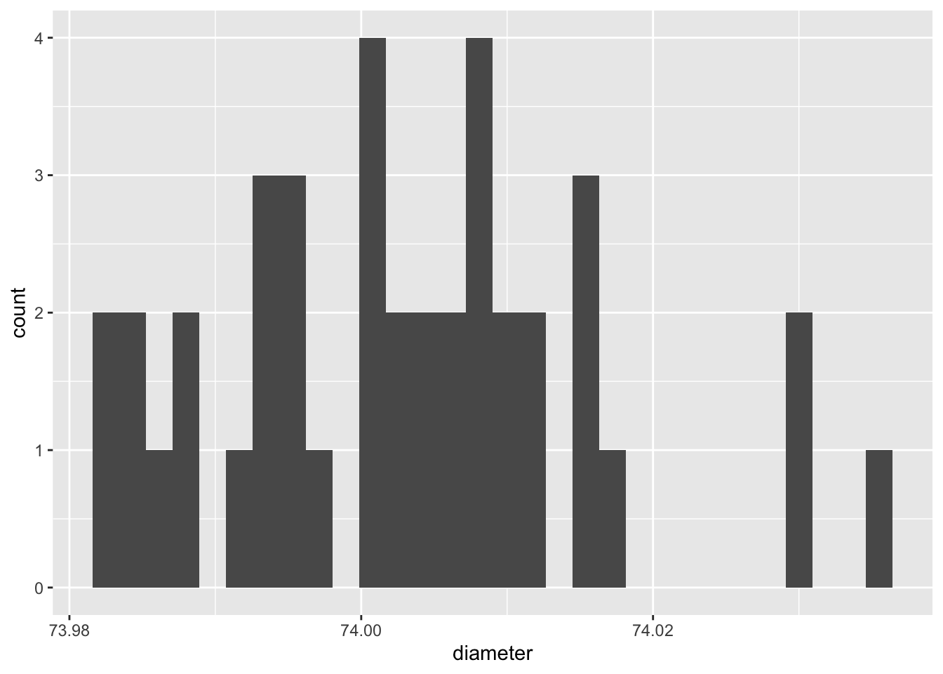
Pareto Chart
Plot Frequency of effect causes, apply 80:20 rule
defect <- c(80, 27, 66, 94, 33)
names(defect) <- c("HA Regulations", "Risk Management", "Data Entry", "Change Management", "IT System Performance")
qcc_pareto <- qcc::paretoChart(defect)
str(qcc_pareto)
## List of 3
## $ call : language qcc::paretoChart(data = defect)
## $ data.name: chr "defect"
## $ tab : num [1:5, 1:4] 94 80 66 33 27 94 174 240 273 300 ...
## ..- attr(*, "dimnames")=List of 2
## .. ..$ defect: chr [1:5] "Change Management" "HA Regulations" "Data Entry" "IT System Performance" ...
## .. ..$ : chr [1:4] "Frequency" "Cum.Freq." "Percentage" "Cum.Percent."
## - attr(*, "class")= chr "paretoChart"plot(qcc_pareto) +
theme(axis.text.x = element_text(angle = 90))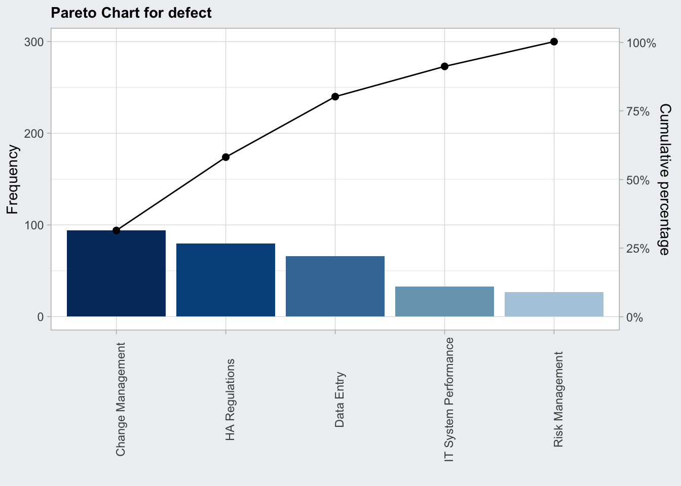
Scatter Plots
- validate established cause and effect relationships
- multivariate control diagrams
Stratification
- identify relevant process subgroups by which to stratify the analysis
- use of process flow charts
Control Charts
- ideally have even sample sizes to obtain even upper and lower control limits, although
qccallow you to create control charts with uneven sample sizes but oc plots cannot be created, thus it is difficult to make good estimates about appropriate sample sizes. - plot in pairs to monitor different summary statistics like x-bar chart (means) and range chart (R chart) as a measure for variance
- use Shewart’s formula to estimate control limits
- phase I determine a calibration period during which the process is in control and determine control limits
- phase II monitor process for out of range values
Continuous Grouped Variables
We are going to measure a continuous variable over time such as the thickness of a board.
Controls Charts use the population standard deviation to flag out of control data points.
Determine population standard deviation:
- determine a calibration period during which the process is in control (set n)
- at each time point measure samples and take the mean
- according to the central limit theorem the distribution of the means will be normally distributed
- measure population standard deviation of the means
sqrt((n-1)/n) * sd(x) - in statistical process control this is considered to be biased
- instead the range and the shewart constant (d2/c4) which depends on the number of measurements (n) are used by the Shewart’s formula to estimate control limits
Determine sample size: - ARL is the average run length (number of consecutive samples) needed to get a point that is outside the upper and lower control limits. For a normal distribution the ARL is 370. So every 370 measurements we will get a false positive signal. - The power of a control chart depends on the sample size. The operator characteristics (OC) plots the probabilty of a false negative (type two error) against the process shift in standard deviations for several sample sizes (n). For a given shift in process deviation we can also determine the probability beta for a false negative using the OC curve. - ARL = 1 / (1 - beta)
X-bar Chart
- Monitors the mean
- uses d2 Shewart’s constants
df## # A tibble: 200 x 3
## diameter sample trial
## <dbl> <int> <lgl>
## 1 74.0 1 TRUE
## 2 74.0 1 TRUE
## 3 74.0 1 TRUE
## 4 74.0 1 TRUE
## 5 74.0 1 TRUE
## 6 74.0 2 TRUE
## 7 74.0 2 TRUE
## 8 74.0 2 TRUE
## 9 74.0 2 TRUE
## 10 74.0 2 TRUE
## # … with 190 more rows# pivot from long to wide
qcc_gr <- qcc::qccGroups(df, diameter, sample)
qcc_gr## [,1] [,2] [,3] [,4] [,5]
## 1 74.030 74.002 74.019 73.992 74.008
## 2 73.995 73.992 74.001 74.011 74.004
## 3 73.988 74.024 74.021 74.005 74.002
## 4 74.002 73.996 73.993 74.015 74.009
## 5 73.992 74.007 74.015 73.989 74.014
## 6 74.009 73.994 73.997 73.985 73.993
## 7 73.995 74.006 73.994 74.000 74.005
## 8 73.985 74.003 73.993 74.015 73.988
## 9 74.008 73.995 74.009 74.005 74.004
## 10 73.998 74.000 73.990 74.007 73.995
## 11 73.994 73.998 73.994 73.995 73.990
## 12 74.004 74.000 74.007 74.000 73.996
## 13 73.983 74.002 73.998 73.997 74.012
## 14 74.006 73.967 73.994 74.000 73.984
## 15 74.012 74.014 73.998 73.999 74.007
## 16 74.000 73.984 74.005 73.998 73.996
## 17 73.994 74.012 73.986 74.005 74.007
## 18 74.006 74.010 74.018 74.003 74.000
## 19 73.984 74.002 74.003 74.005 73.997
## 20 74.000 74.010 74.013 74.020 74.003
## 21 73.988 74.001 74.009 74.005 73.996
## 22 74.004 73.999 73.990 74.006 74.009
## 23 74.010 73.989 73.990 74.009 74.014
## 24 74.015 74.008 73.993 74.000 74.010
## 25 73.982 73.984 73.995 74.017 74.013
## 26 74.012 74.015 74.030 73.986 74.000
## 27 73.995 74.010 73.990 74.015 74.001
## 28 73.987 73.999 73.985 74.000 73.990
## 29 74.008 74.010 74.003 73.991 74.006
## 30 74.003 74.000 74.001 73.986 73.997
## 31 73.994 74.003 74.015 74.020 74.004
## 32 74.008 74.002 74.018 73.995 74.005
## 33 74.001 74.004 73.990 73.996 73.998
## 34 74.015 74.000 74.016 74.025 74.000
## 35 74.030 74.005 74.000 74.016 74.012
## 36 74.001 73.990 73.995 74.010 74.024
## 37 74.015 74.020 74.024 74.005 74.019
## 38 74.035 74.010 74.012 74.015 74.026
## 39 74.017 74.013 74.036 74.025 74.026
## 40 74.010 74.005 74.029 74.000 74.020q1 <- qcc(
qcc_gr[1:25, ],
type = "xbar",
newdata = qcc_gr[26:nrow(qcc_gr), ],
rules = c(1, 2, 3, 4)
)
q1## ── Quality Control Chart ─────────────────────────
##
## Chart type = xbar
## Data (phase I) = qcc_gr[1:25, ]
## Number of groups = 25
## Group sample size = 5
## Center of group statistics = 74.00118
## Standard deviation = 0.009785039
##
## New data (phase II) = qcc_gr[26:nrow(qcc_gr), ]
## Number of groups = 15
## Group sample size = 5
##
## Control limits at nsigmas = 3
## LCL UCL
## 73.98805 74.0143plot(q1)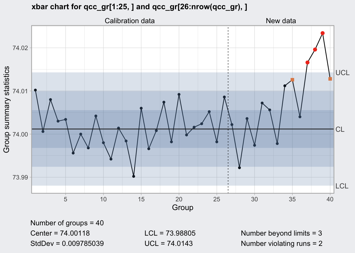
q1_oc <- qcc::ocCurves(q1)

q1_oc
## ── Operating Characteristic Curves ───────────────
##
## Chart type = xbar
## Prob. type II error (beta) =
## sample size
## shift (StdDev) 1 5 10 15 20
## 0.0 0.9973 0.9973 0.9973 0.9973 0.9973
## 0.1 0.9972 0.9966 0.9959 0.9952 0.9944
## 0.2 0.9968 0.9944 0.9909 0.9869 0.9823
## :
## 4.9 0.0287 0.0000 0.0000 0.0000 0.0000
## 5.0 0.0228 0.0000 0.0000 0.0000 0.0000
## Average run length (ARL) =
## sample size
## shift (StdDev) 1 5 10 15 20
## 0.0 370 370 370 370 370
## 0.1 353 296 244 206 178
## 0.2 308 178 110 76 57
## :
## 4.9 1 1 1 1 1
## 5.0 1 1 1 1 1plot(q1_oc)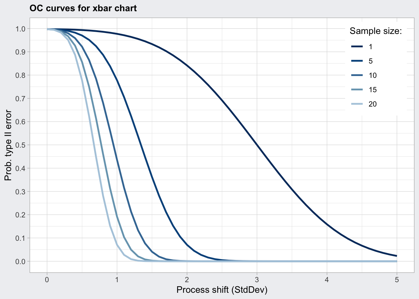
arl_n5 <- q1_oc$ARL %>%
  as_tibble(rownames = "shift_stdev") %>%
  filter(shift_stdev == "1.0") %>%
  pull(`5`)

arl_n5
## [1] 4.495312So for a change in average diameter by 0.009785 we need in average 4.4953122 runs to detect a change in the mean statistic using 5 samples.
R Chart
- monitors process stability by means of the sample ranges
- uses d3 and d2 Shewart’s constants
- appropriate for sample sizes < 8
q2 <- qcc(
  qcc_gr[1:25, ],
  type = "R",
  newdata = qcc_gr[26:nrow(qcc_gr), ],
  rules = c(1, 2, 3, 4)
)

q2
## ── Quality Control Chart ─────────────────────────
##
## Chart type = R
## Data (phase I) = qcc_gr[1:25, ]
## Number of groups = 25
## Group sample size = 5
## Center of group statistics = 0.02276
## Standard deviation = 0.009785039
##
## New data (phase II) = qcc_gr[26:nrow(qcc_gr), ]
## Number of groups = 15
## Group sample size = 5
##
## Control limits at nsigmas = 3
## LCL UCL
## 0 0.04812533plot(q2)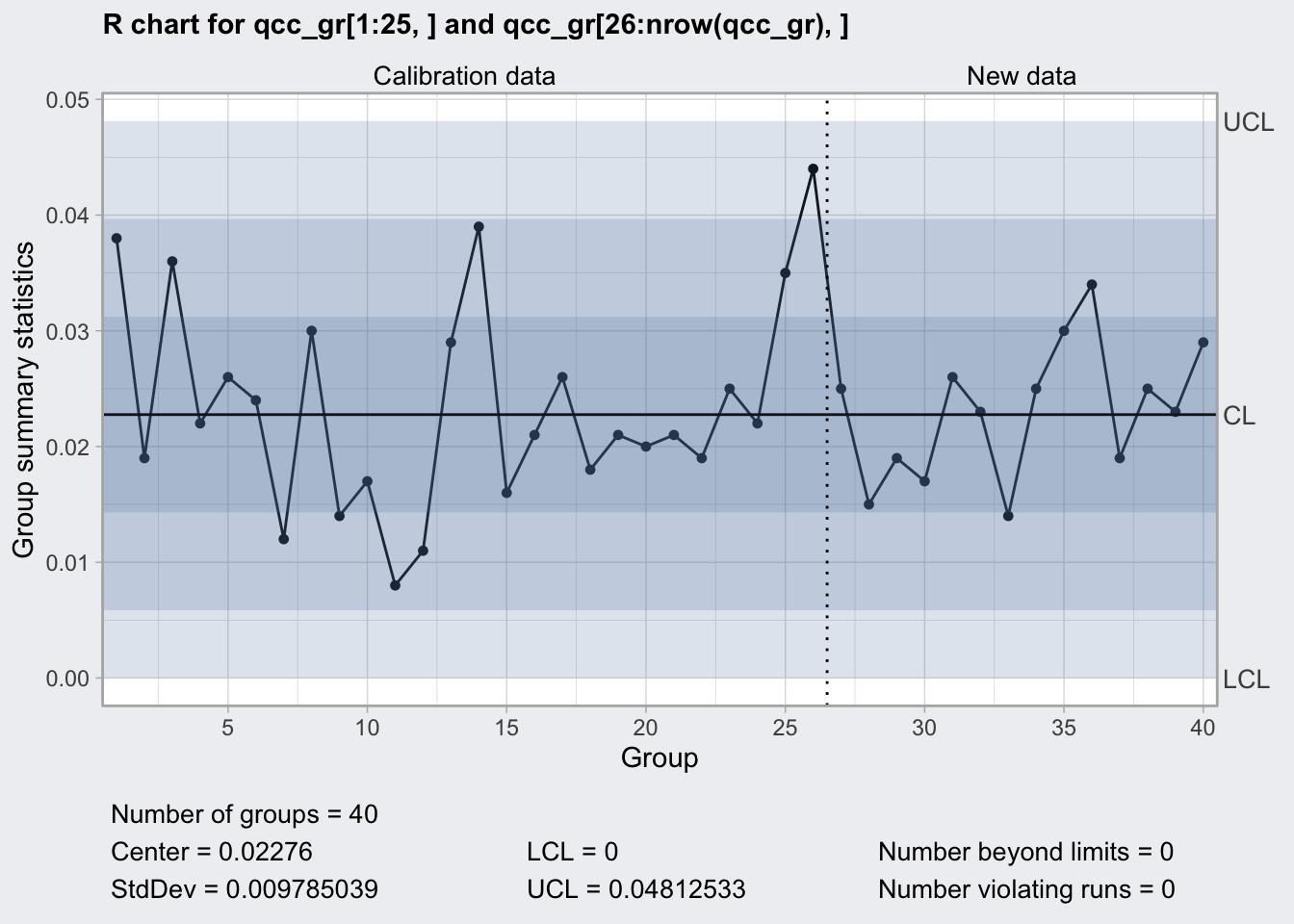
q2_oc <- qcc::ocCurves(q2)

# throws error, https://github.com/luca-scr/qcc/issues/31
# plot(q2_oc)

q2_oc
## ── Operating Characteristic Curves ───────────────
##
## Chart type = R
## Prob. type II error (beta) =
## sample size
## scale multiplier 2 5 10 15 20
## 1.0 0.9908 0.9954 0.9956 0.9955 0.9954
## 1.1 0.9822 0.9864 0.9841 0.9818 0.9798
## 1.2 0.9701 0.9692 0.9583 0.9486 0.9403
## :
## 5.9 0.3413 0.0233 0.0003 0.0000 0.0000
## 6.0 0.3360 0.0219 0.0002 0.0000 0.0000
## Average run length (ARL) =
## sample size
## scale multiplier 2 5 10 15 20
## 1.0 109 217 229 223 217
## 1.1 56 74 63 55 50
## 1.2 33 32 24 19 17
## :
## 5.9 2 1 1 1 1
## 6.0 2 1 1 1 1arl_n5 <- q2_oc$ARL %>%
as_tibble(rownames = "scale_multiplier") %>%
filter(scale_multiplier == "1.5") %>%
pull(`5`)
arl_n5## [1] 7.198125So for a change in range by 50% need in average 7.1981249 runs using 5 samples.
S Chart
- monitors process stability by means of standard deviations
- uses c4 Shewart’s constant
- appropriate for sample sizes >= 8
q3 <- qcc(
  qcc_gr[1:25, ],
  type = "S",
  newdata = qcc_gr[26:nrow(qcc_gr), ],
  rules = c(1, 2, 3, 4)
)

q3
## ── Quality Control Chart ─────────────────────────
##
## Chart type = S
## Data (phase I) = qcc_gr[1:25, ]
## Number of groups = 25
## Group sample size = 5
## Center of group statistics = 0.009240037
## Standard deviation = 0.009829977
##
## New data (phase II) = qcc_gr[26:nrow(qcc_gr), ]
## Number of groups = 15
## Group sample size = 5
##
## Control limits at nsigmas = 3
## LCL UCL
## 0 0.01930242plot(q3)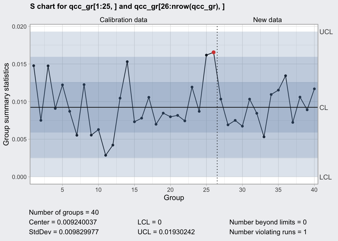
q3_oc <- qcc::ocCurves(q3)

# throws error, https://github.com/luca-scr/qcc/issues/31
# plot(q3_oc)

q3_oc
## ── Operating Characteristic Curves ───────────────
##
## Chart type = S
## Prob. type II error (beta) =
## sample size
## scale multiplier 2 5 10 15 20
## 1.0 0.9908 0.9961 0.9970 0.9972 0.9972
## 1.1 0.9822 0.9874 0.9860 0.9838 0.9812
## 1.2 0.9701 0.9700 0.9574 0.9425 0.9261
## :
## 5.9 0.3413 0.0212 0.0001 0.0000 0.0000
## 6.0 0.3360 0.0199 0.0001 0.0000 0.0000
## Average run length (ARL) =
## sample size
## scale multiplier 2 5 10 15 20
## 1.0 109 256 333 351 358
## 1.1 56 79 72 62 53
## 1.2 33 33 23 17 14
## :
## 5.9 2 1 1 1 1
## 6.0 2 1 1 1 1arl_n5 <- q3_oc$ARL %>%
as_tibble(rownames = "scale_multiplier") %>%
filter(scale_multiplier == "1.5") %>%
pull(`5`)So for a change in range by 50% need in average 6.9559271 runs using 5 samples.
Continuous Non-Grouped Variables
If a process is described best by a continuous one at a time measurement we cannot use sampling
- central limit theorem does not apply
- normality needs to be confirmed
- if possible use power transformation to normalize
- accompany x-bar chart with moving range chart
X-bar chart
- uses the moving range to calculate global standard deviation
- takes Shewart’s constant d2 for n = 2
# airplane paint viscosity, one batch takes hours to produce and no rational subgroups can be formed
data("viscosity")
df_vis <- viscosity

df_vis
## batch viscosity trial
## 1 1 34.05 TRUE
## 2 2 34.40 TRUE
## 3 3 33.59 TRUE
## 4 4 35.96 TRUE
## 5 5 34.70 TRUE
## 6 6 33.51 TRUE
## 7 7 33.79 TRUE
## 8 8 34.04 TRUE
## 9 9 34.52 TRUE
## 10 10 33.75 TRUE
## 11 11 33.27 TRUE
## 12 12 33.71 TRUE
## 13 13 34.03 TRUE
## 14 14 34.58 TRUE
## 15 15 34.02 TRUE
## 16 16 33.97 TRUE
## 17 17 34.05 TRUE
## 18 18 34.04 TRUE
## 19 19 33.73 TRUE
## 20 20 34.05 TRUE
## 21 21 34.39 FALSE
## 22 22 33.75 FALSE
## 23 23 33.40 FALSE
## 24 24 33.27 FALSE
## 25 25 34.65 FALSE
## 26 26 34.80 FALSE
## 27 27 34.55 FALSE
## 28 28 35.40 FALSE
## 29 29 34.75 FALSE
## 30 30 34.50 FALSE
## 31 31 34.70 FALSE
## 32 32 34.29 FALSE
## 33 33 34.61 FALSE
## 34 34 34.49 FALSE
## 35 35 35.03 FALSEq4 <- qcc(
df_vis$viscosity[df_vis$trial],
type = "xbar.one",
newdata = df_vis$viscosity[! df_vis$trial],
rules = c(1, 2, 3, 4)
)
q4## ── Quality Control Chart ─────────────────────────
##
## Chart type = xbar.one
## Data (phase I) = df_vis$viscosity[df_vis$trial]
## Number of groups = 20
## Group sample size = 1
## Center of group statistics = 34.088
## Standard deviation = 0.5076521
##
## New data (phase II) = df_vis$viscosity[!df_vis$trial]
## Number of groups = 15
## Group sample size = 1
##
## Control limits at nsigmas = 3
## LCL UCL
## 32.56504 35.61096plot(q4)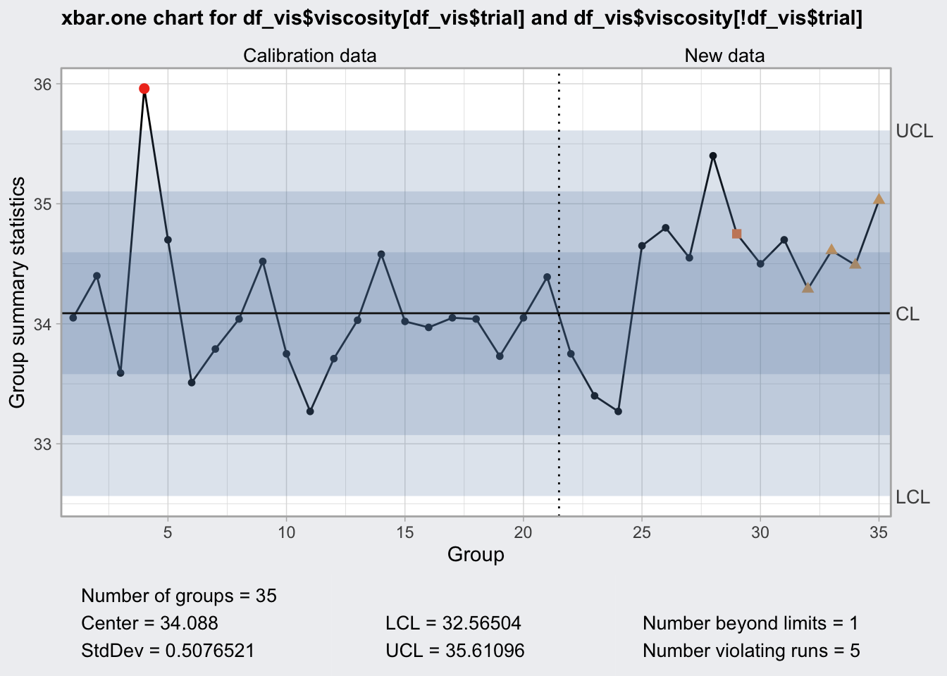
R Chart
- uses the range between a given and the next measurement
vis_mat <- df_vis %>%
  mutate(lead = lead(viscosity)) %>%
  select(viscosity, lead) %>%
  filter(! is.na(lead)) %>%
  as.matrix()


q5 <- qcc(
  vis_mat[df_vis$trial[1:nrow(df_vis)-1], ],
  type = "R",
  newdata = vis_mat[! df_vis$trial[1:nrow(df_vis)-1], ]
)

q5
## ── Quality Control Chart ─────────────────────────
##
## Chart type = R
## Data (phase I) = vis_mat[df_vis$trial[1:nrow(df_vis) - 1], ]
## Number of groups = 20
## Group sample size = 2
## Center of group statistics = 0.561
## Standard deviation = 0.4973404
##
## New data (phase II) = vis_mat[!df_vis$trial[1:nrow(df_vis) - 1], ]
## Number of groups = 14
## Group sample size = 2
##
## Control limits at nsigmas = 3
## LCL UCL
## 0 1.832953plot(q5)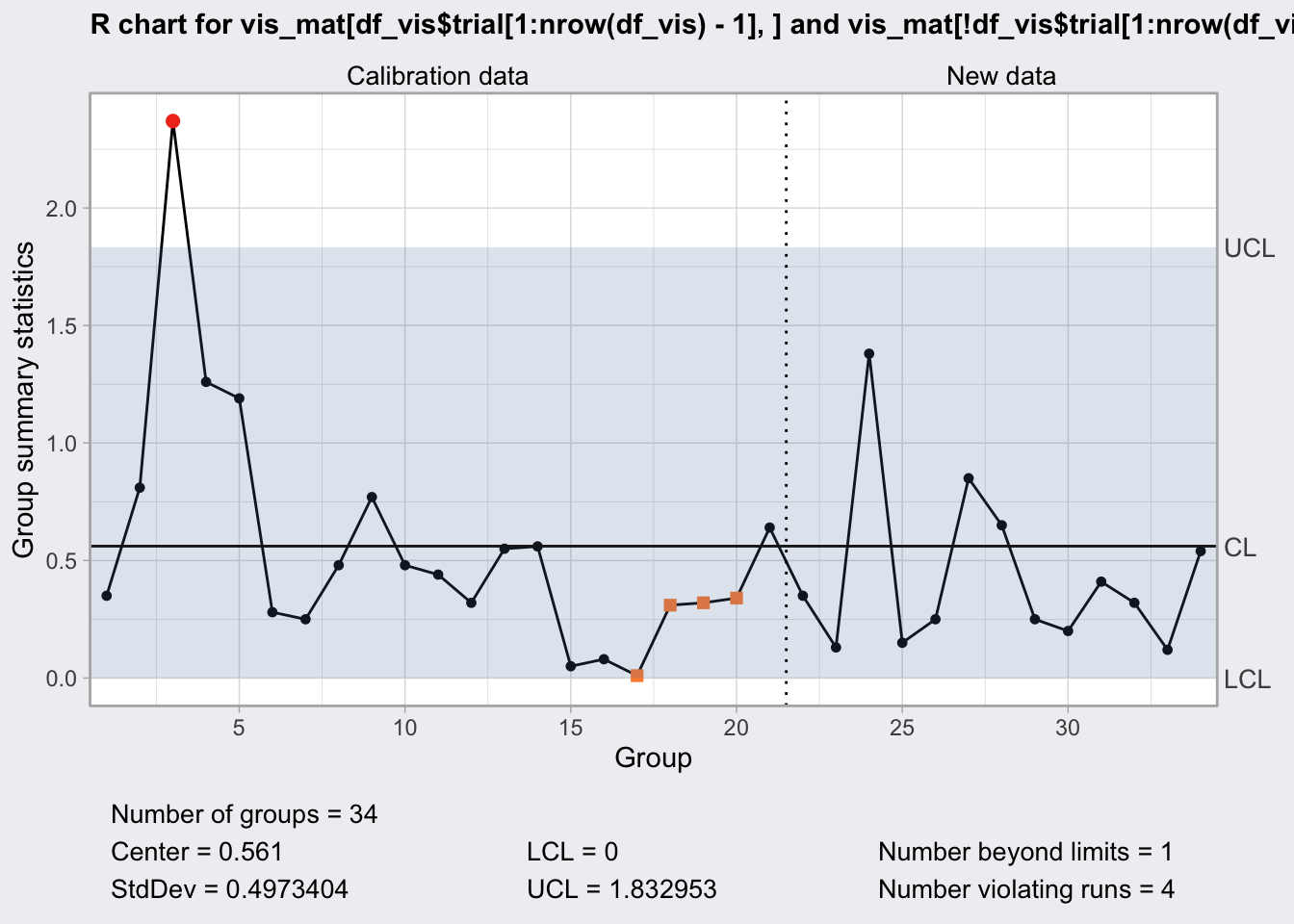
Discrete Measurements
p and np Charts
- measure frequency or relative frequency
- p is for relative frequency
- np for frequency
data("orangejuice")
df_oj <- orangejuice

q6 <- qcc(
  df_oj$D[df_oj$trial],
  df_oj$size[df_oj$trial],
  type = "p",
  newdata = df_oj$D[! df_oj$trial],
  newsizes = df_oj$size[! df_oj$trial],
  rules = c(1, 2, 3, 4)
)

q6
## ── Quality Control Chart ─────────────────────────
##
## Chart type = p
## Data (phase I) = df_oj$D[df_oj$trial]
## Number of groups = 30
## Group sample size = 50
## Center of group statistics = 0.2313333
## Standard deviation = 0.05963526
##
## New data (phase II) = df_oj$D[!df_oj$trial]
## Number of groups = 24
## Group sample size = 50
##
## Control limits at nsigmas = 3
## LCL UCL
## 0.05242755 0.4102391
## 0.05242755 0.4102391
## :
## 0.05242755 0.4102391plot(q6)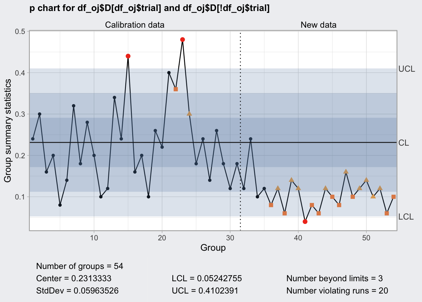
q6_oc <- qcc::ocCurves(q6)

q6_oc
## ── Operating Characteristic Curves ───────────────
##
## Chart type = p
## Prob. type II error (beta) =
##
## fraction nonconforming [,1]
## 0.00 0.0000
## 0.01 0.0894
## 0.02 0.2642
## :
## 0.99 0.0000
## 1.00 0.0000
## Average run length (ARL) =
##
## fraction nonconforming [,1]
## 0.00 1
## 0.01 1
## 0.02 1
## :
## 0.99 1
## 1.00 1plot(q6_oc)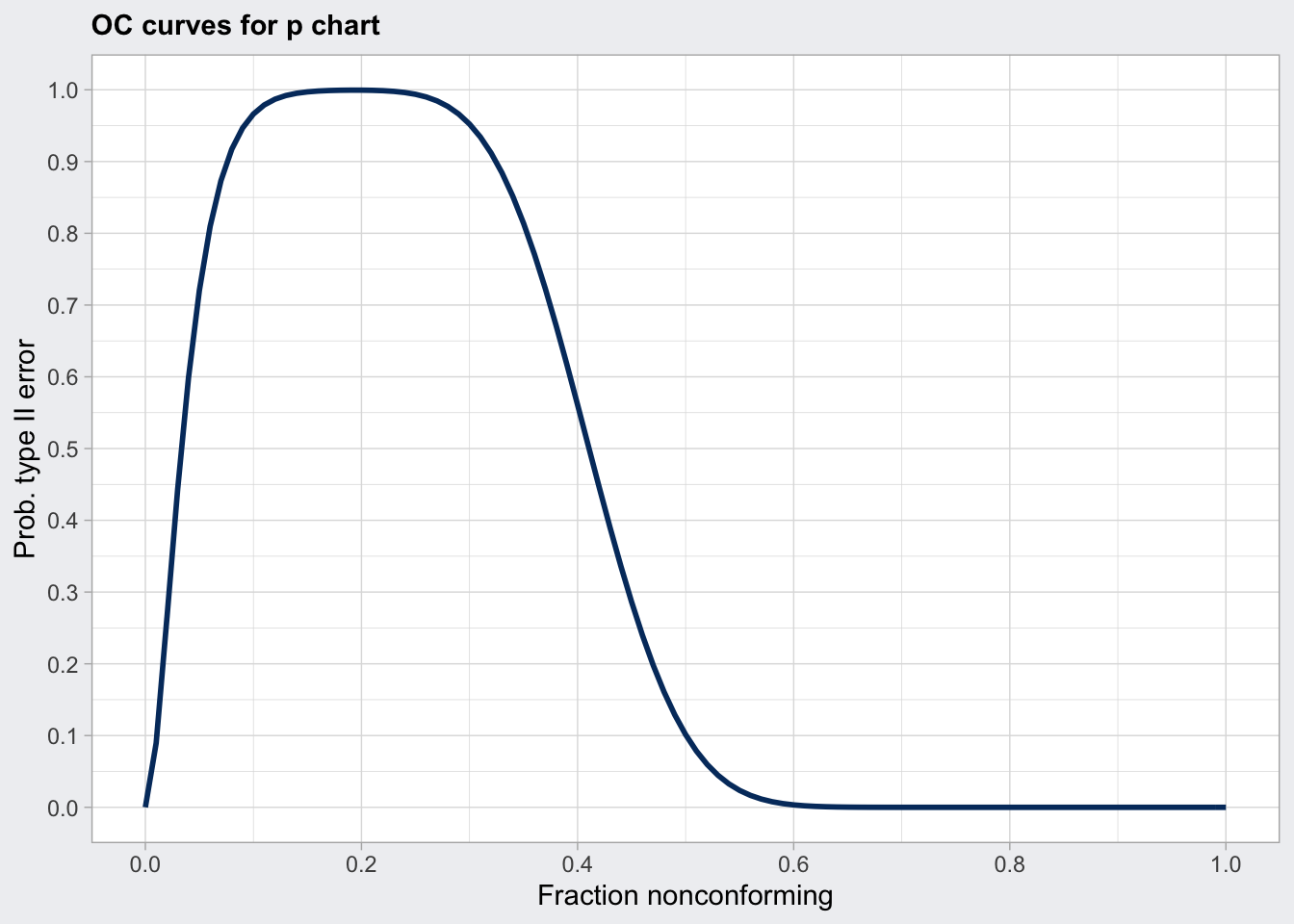
plot(q6_oc, what = "ARL")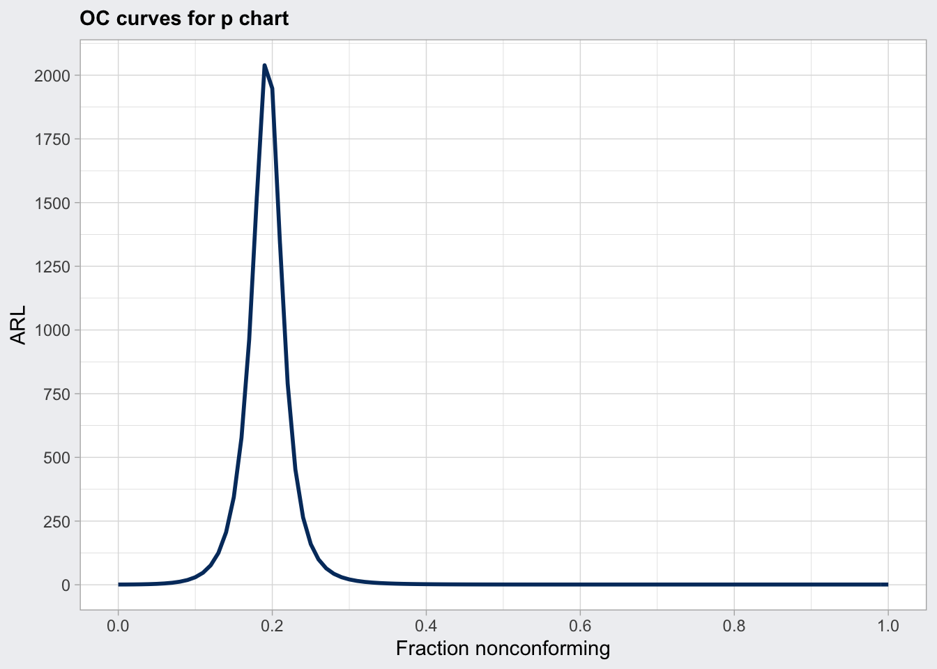
q6a <- qcc(
  df_oj$D[df_oj$trial],
  df_oj$size[df_oj$trial],
  type = "np",
  newdata = df_oj$D[! df_oj$trial],
  newsizes = df_oj$size[! df_oj$trial],
  rules = c(1, 2, 3, 4)
)

q6a
## ── Quality Control Chart ─────────────────────────
##
## Chart type = np
## Data (phase I) = df_oj$D[df_oj$trial]
## Number of groups = 30
## Group sample size = 50
## Center of group statistics = 11.56667
## Standard deviation = 2.981763
##
## New data (phase II) = df_oj$D[!df_oj$trial]
## Number of groups = 24
## Group sample size = 50
##
## Control limits at nsigmas = 3
## LCL UCL
## 2.621377 20.51196plot(q6a)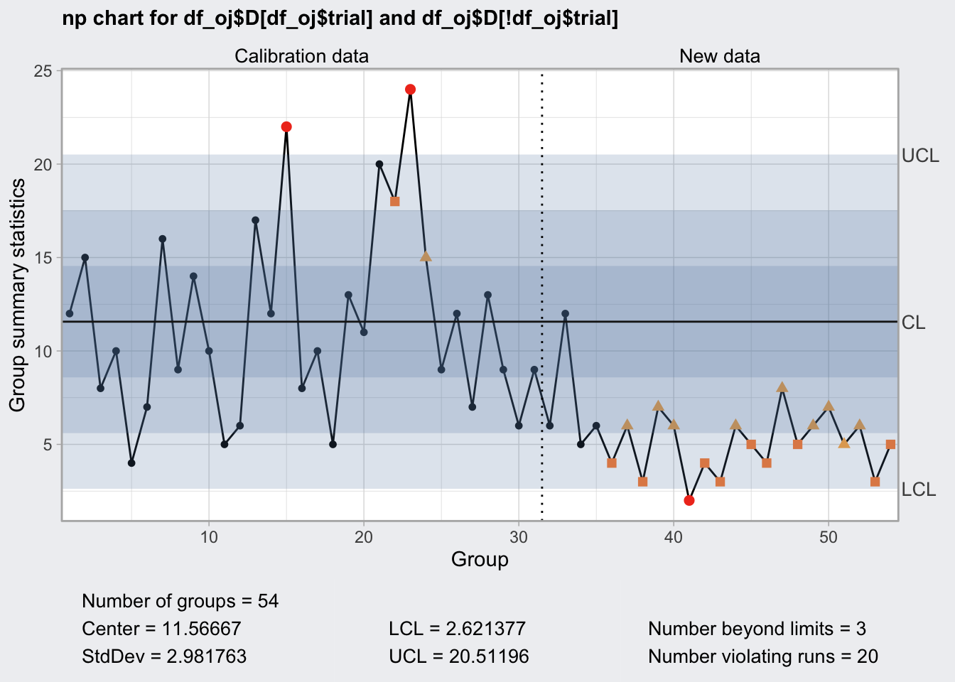
c chart
- for count of events that cannot be attributed to a sample size
- examples: nonconformities per day, defects per m^2 of fabric or flaws per metal plate
- unit should stay constant
library(SixSigma)

ss.data.thickness2 %>%
  head(15)
## day shift thickness ushift flaws
## 1 1 1 0.713 1.1 9
## 2 1 1 0.776 1.1 NA
## 3 1 1 0.743 1.1 NA
## 4 1 1 0.713 1.1 NA
## 5 1 1 0.747 1.1 NA
## 6 1 1 0.753 1.1 NA
## 7 1 2 0.749 1.2 2
## 8 1 2 0.726 1.2 7
## 9 1 2 0.774 1.2 9
## 10 1 2 0.744 1.2 NA
## 11 1 2 0.718 1.2 NA
## 12 1 2 0.677 1.2 NA
## 13 2 1 0.778 2.1 7
## 14 2 1 0.802 2.1 NA
## 15 2 1 0.798 2.1 NA# remove uninspected items
df_flaws <- ss.data.thickness2 %>%
as_tibble() %>%
filter(! is.na(flaws))
df_flaws## # A tibble: 23 x 5
## day shift thickness ushift flaws
## <fct> <fct> <dbl> <chr> <int>
## 1 1 1 0.713 1.1 9
## 2 1 2 0.749 1.2 2
## 3 1 2 0.726 1.2 7
## 4 1 2 0.774 1.2 9
## 5 2 1 0.778 2.1 7
## 6 2 2 0.78 2.2 4
## 7 2 2 0.729 2.2 6
## 8 2 2 0.793 2.2 9
## 9 3 1 0.775 3.1 9
## 10 3 2 0.727 3.2 4
## # … with 13 more rowsq7 <- qcc(
df_flaws$flaws,
type = "c",
rules = c(1, 2, 3, 4)
)
q7## ── Quality Control Chart ─────────────────────────
##
## Chart type = c
## Data (phase I) = df_flaws$flaws
## Number of groups = 23
## Group sample size = 1
## Center of group statistics = 5.26087
## Standard deviation = 2.293659
##
## Control limits at nsigmas = 3
## LCL UCL
## 0 12.14185plot(q7)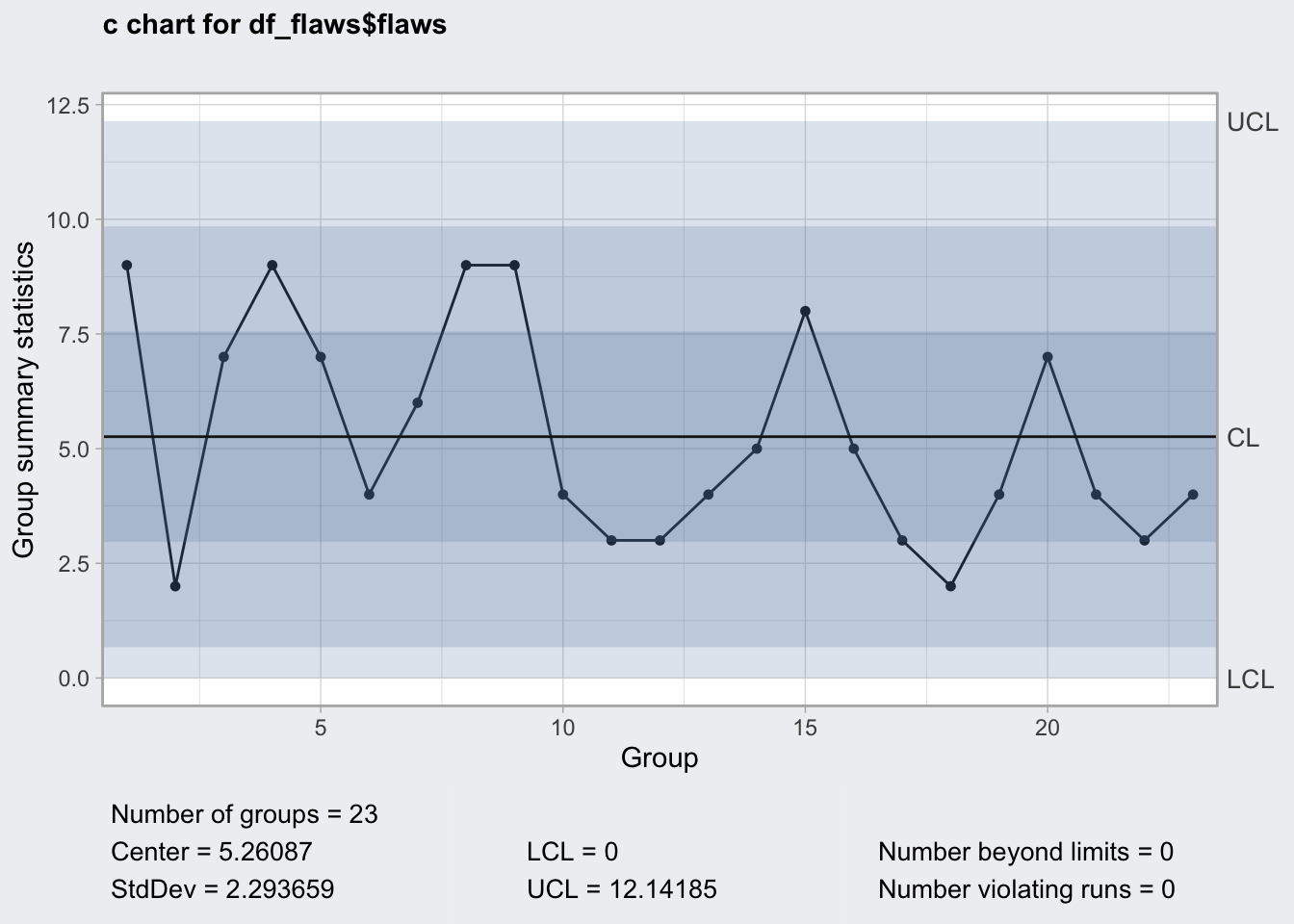
q7_oc <- qcc::ocCurves(q7)

q7_oc
## ── Operating Characteristic Curves ───────────────
##
## Chart type = c
## Prob. type II error (beta) =
## [,1]
## 0.00 1e+00
## 1.00 1e+00
## 2.00 1e+00
## :
## 28.00 6e-04
## 29.00 3e-04
## Average run length (ARL) =
## [,1]
## 0.00 Inf
## 1.00 15723815904
## 2.00 4822834
## :
## 28.00 1
## 29.00 1plot(q7_oc, what = "ARL") +
coord_cartesian(ylim = c(0, 10))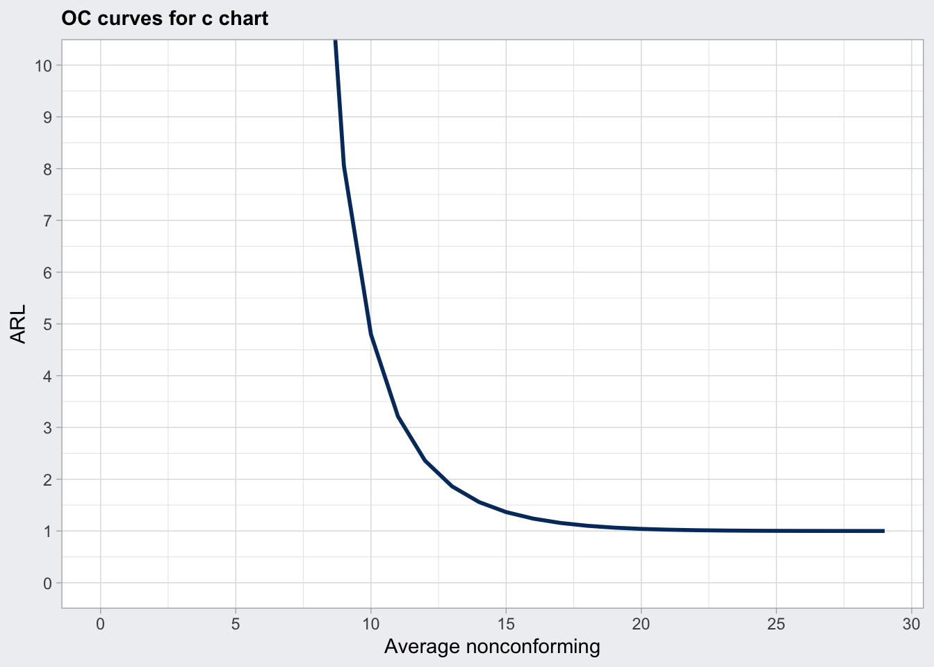
u chart
- average number of defects from a varying number of samples
- for example: 18 flaws from 3 metal plates, then 3 flaws in 5 metal plates
df_gr_flaws <- df_flaws %>%
  group_by(ushift) %>%
  summarise(n_plates_per_shift = n(),
            n_flaws_per_shift = sum(flaws))

df_gr_flaws
## # A tibble: 14 x 3
## ushift n_plates_per_shift n_flaws_per_shift
## <chr> <int> <int>
## 1 1.1 1 9
## 2 1.2 3 18
## 3 2.1 1 7
## 4 2.2 3 19
## 5 3.1 1 9
## 6 3.2 1 4
## 7 4.1 2 6
## 8 4.2 1 4
## 9 5.1 1 5
## 10 5.2 2 13
## 11 6.1 2 5
## 12 6.2 1 4
## 13 7.1 1 7
## 14 7.2 3 11qu8 <- qcc(
df_gr_flaws$n_flaws_per_shift,
type = "u",
sizes = df_gr_flaws$n_plates_per_shift,
rules = c(1, 2, 3, 4)
)
qu8## ── Quality Control Chart ─────────────────────────
##
## Chart type = u
## Data (phase I) = df_gr_flaws$n_flaws_per_shift
## Number of groups = 14
## Group sample sizes =
## sizes 1 2 3
## counts 8 3 3
## Center of group statistics = 5.26087
## Standard deviation = 2.293659
##
## Control limits at nsigmas = 3
## LCL UCL
## 0.000000 12.141845
## 1.288136 9.233603
## :
## 1.288136 9.233603plot(qu8)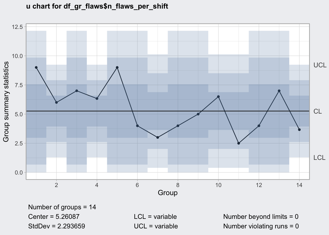
# OC curves need constant sample sizes
# qu8_oc <- qcc::ocCurves(qu8)
Capability/Performance Indices
measure whether consumer specified upper and lower specification limits (LSL/USL) are compatible with process control limits (LCL/UCL)
performance measures long-term variability and capacity short-term variability
C = (USL - LSL) / 6sigma
index below 1 is unsufficient, 1.33-167 is outstanding and 2 refers to six sigma quality
adjusted index variations account for processes that are not perfectly centered
Cp: capability index
Cp_l: lower index
Cp_u: upper index
Cp_k: minimum of lower and upper index
Cpm : Tagauchi index (controls for not centered processes)
q1## ── Quality Control Chart ─────────────────────────
##
## Chart type = xbar
## Data (phase I) = qcc_gr[1:25, ]
## Number of groups = 25
## Group sample size = 5
## Center of group statistics = 74.00118
## Standard deviation = 0.009785039
##
## New data (phase II) = qcc_gr[26:nrow(qcc_gr), ]
## Number of groups = 15
## Group sample size = 5
##
## Control limits at nsigmas = 3
## LCL UCL
## 73.98805 74.0143q1_pc <- qcc::processCapability(q1, spec.limits = c(73.975, 74.025))
q1_pc## ── Process Capability Analysis ───────────────────
##
## Number of obs = 125 Target = 74
## Center = 74.00118 LSL = 73.975
## StdDev = 0.009785039 USL = 74.025
##
## Capability indices Value 2.5% 97.5%
## Cp 0.852 0.746 0.957
## Cp_l 0.892 0.786 0.997
## Cp_u 0.812 0.714 0.910
## Cp_k 0.812 0.695 0.928
## Cpm 0.846 0.740 0.951
##
## Exp<LSL 0.0037% Obs<LSL 0.008%
## Exp>USL 0.0075% Obs>USL 0.008%plot(q1_pc)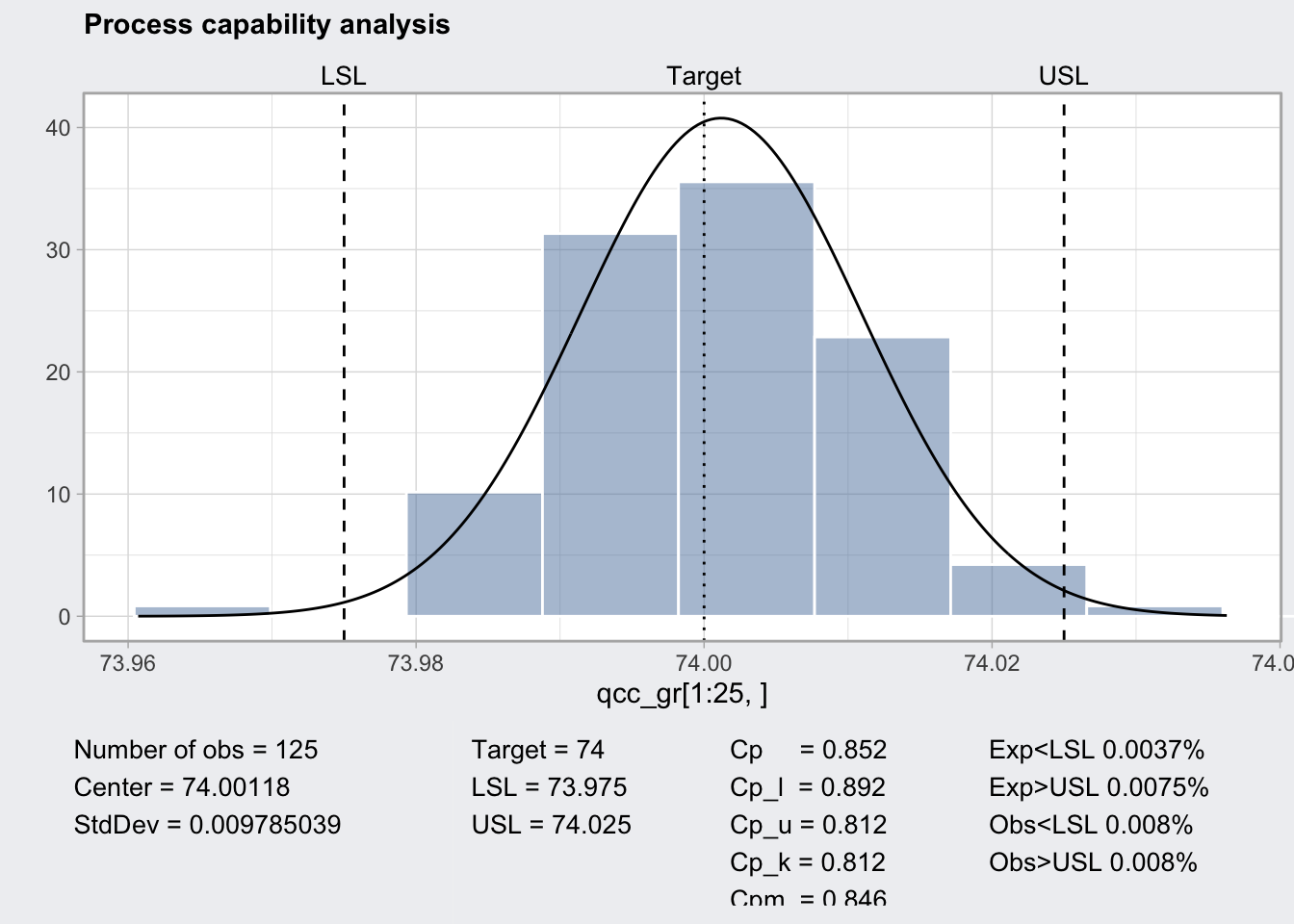
q1_pc <- qcc::processCapability(q1, spec.limits = c(73.95, 74.05))

q1_pc
## ── Process Capability Analysis ───────────────────
##
## Number of obs = 125 Target = 74
## Center = 74.00118 LSL = 73.95
## StdDev = 0.009785039 USL = 74.05
##
## Capability indices Value 2.5% 97.5%
## Cp 1.70 1.49 1.91
## Cp_l 1.74 1.55 1.93
## Cp_u 1.66 1.48 1.84
## Cp_k 1.66 1.45 1.88
## Cpm 1.69 1.48 1.90
##
## Exp<LSL 0% Obs<LSL 0%
## Exp>USL 0% Obs>USL 0%plot(q1_pc)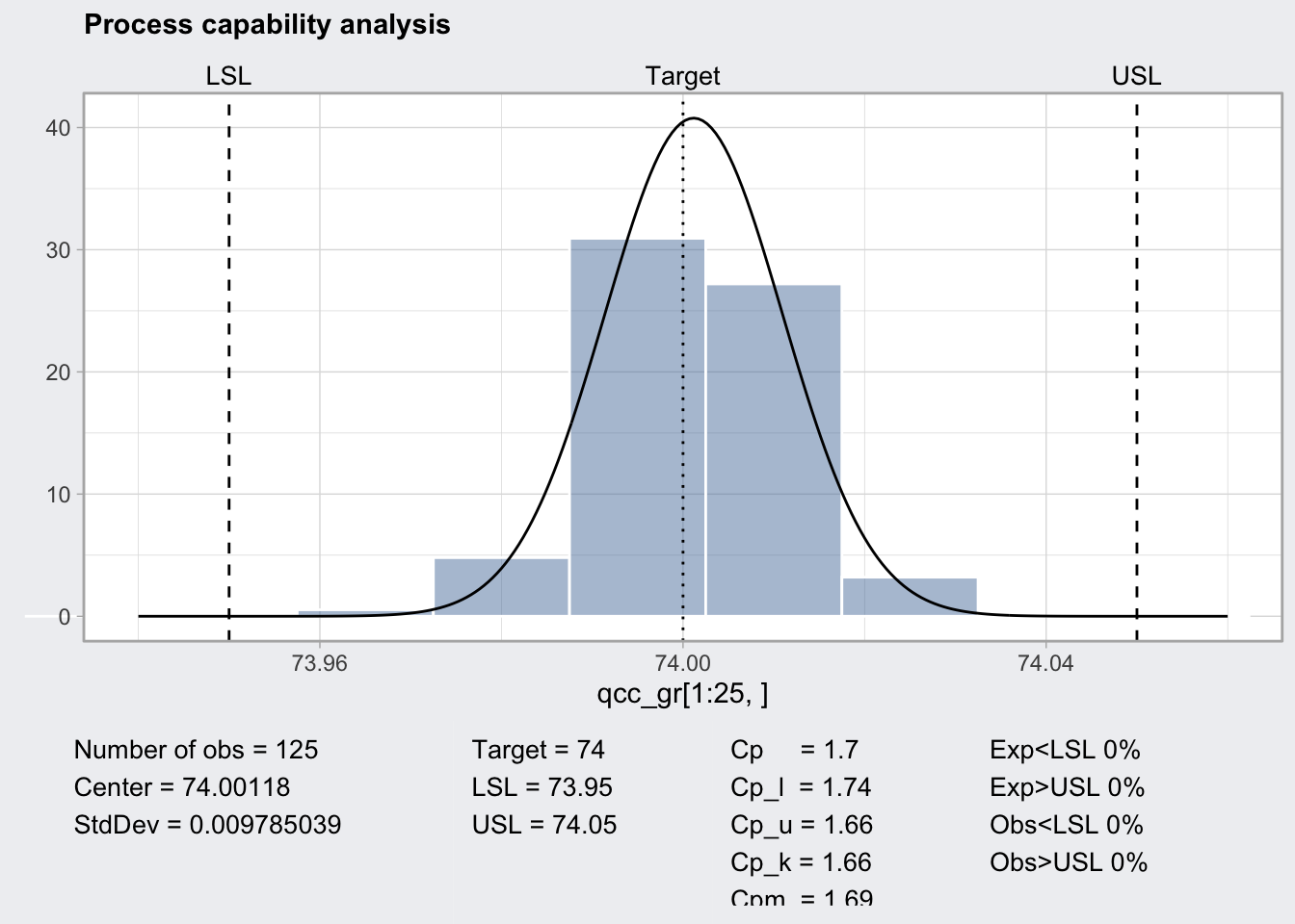
CUSUM Chart
- cumulative sum chart
- two lines one below zero and one above zero and a center which is the expected value.
- positive deviation of the process from the central value results in an uptick of both lines
- negative deviation of the process from the central value results in a down tick of both lines
- both lines never cross the central line
- supposedly more sensitive than regular control charts
qcc_gr## [,1] [,2] [,3] [,4] [,5]
## 1 74.030 74.002 74.019 73.992 74.008
## 2 73.995 73.992 74.001 74.011 74.004
## 3 73.988 74.024 74.021 74.005 74.002
## 4 74.002 73.996 73.993 74.015 74.009
## 5 73.992 74.007 74.015 73.989 74.014
## 6 74.009 73.994 73.997 73.985 73.993
## 7 73.995 74.006 73.994 74.000 74.005
## 8 73.985 74.003 73.993 74.015 73.988
## 9 74.008 73.995 74.009 74.005 74.004
## 10 73.998 74.000 73.990 74.007 73.995
## 11 73.994 73.998 73.994 73.995 73.990
## 12 74.004 74.000 74.007 74.000 73.996
## 13 73.983 74.002 73.998 73.997 74.012
## 14 74.006 73.967 73.994 74.000 73.984
## 15 74.012 74.014 73.998 73.999 74.007
## 16 74.000 73.984 74.005 73.998 73.996
## 17 73.994 74.012 73.986 74.005 74.007
## 18 74.006 74.010 74.018 74.003 74.000
## 19 73.984 74.002 74.003 74.005 73.997
## 20 74.000 74.010 74.013 74.020 74.003
## 21 73.988 74.001 74.009 74.005 73.996
## 22 74.004 73.999 73.990 74.006 74.009
## 23 74.010 73.989 73.990 74.009 74.014
## 24 74.015 74.008 73.993 74.000 74.010
## 25 73.982 73.984 73.995 74.017 74.013
## 26 74.012 74.015 74.030 73.986 74.000
## 27 73.995 74.010 73.990 74.015 74.001
## 28 73.987 73.999 73.985 74.000 73.990
## 29 74.008 74.010 74.003 73.991 74.006
## 30 74.003 74.000 74.001 73.986 73.997
## 31 73.994 74.003 74.015 74.020 74.004
## 32 74.008 74.002 74.018 73.995 74.005
## 33 74.001 74.004 73.990 73.996 73.998
## 34 74.015 74.000 74.016 74.025 74.000
## 35 74.030 74.005 74.000 74.016 74.012
## 36 74.001 73.990 73.995 74.010 74.024
## 37 74.015 74.020 74.024 74.005 74.019
## 38 74.035 74.010 74.012 74.015 74.026
## 39 74.017 74.013 74.036 74.025 74.026
## 40 74.010 74.005 74.029 74.000 74.020q1 <- qcc(
qcc_gr[1:25, ],
type = "xbar",
newdata = qcc_gr[26:nrow(qcc_gr), ],
rules = c(1, 2, 3, 4)
)
plot(q1)
q9 <- qcc::cusum(
  qcc_gr[1:25, ],
  newdata = qcc_gr[26:nrow(qcc_gr), ]
)

plot(q9)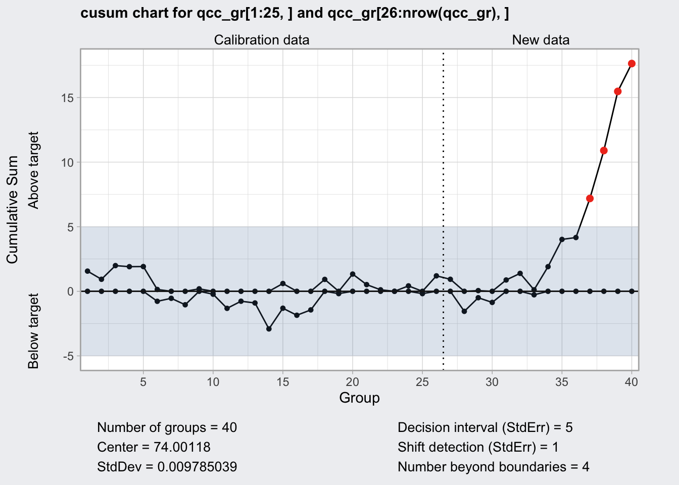
EWMA Chart
- exponentially weighted moving average chart
- zj = gamma * xj + (1 - gamma) * zj-1
- if the smoothing parameter gamma is 0.2 a given value for x is 20% present value and 80% past values
+indicates the actual values- supposed to work well for not normal values
q10 <- qcc::ewma(
  qcc_gr[1:25, ],
  newdata = qcc_gr[26:nrow(qcc_gr), ]
)

plot(q10)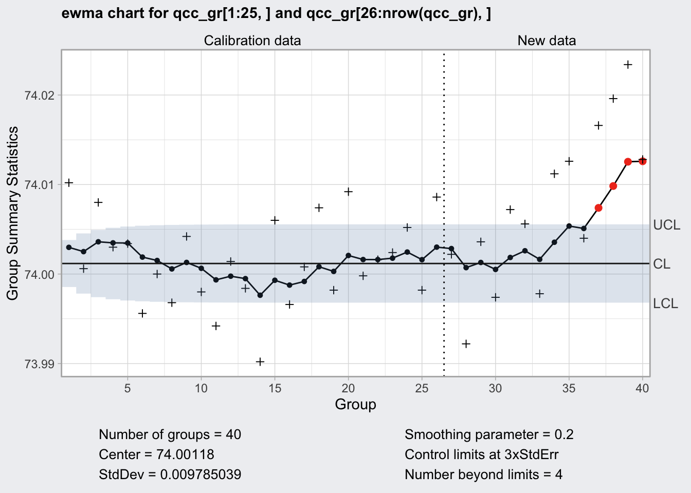
Sampling/Stratification
Naturally samples need to be representative of the population. If there are known subgroups it is important to adapt a stratified sampling strategy.
Attribute Acceptance Sampling
- attribute: defective / not defective
- producer wants a high probability of acceptance for a lot with a low defective fraction
- producers and consumer agree on acceptable quality level (AQL)
- alpha (producers risk) is the probability with which a lot that passes AQL is rejected
- consumer wants a high probability of rejection for a lot with a high defective ratio
- producers and consumer agree on lot tolerance percent defective (LTPD)
- beta (consumers risk) is the probability with which a lot that does not pass LTPD is accepted
Requirements:
- AQL: 0.06
- alpha: 0.05
- LTPD: 0.16
- beta: 0.10
library(AcceptanceSampling)

plan <- AcceptanceSampling::find.plan(
  PRP = c(0.06, 0.95),
  CRP = c(0.16, 0.10)
)

plan
## $n
## [1] 79
##
## $c
## [1] 8
##
## $r
## [1] 9oc <- AcceptanceSampling::OC2c(plan$n, plan$c, plan$r)
plot(oc, xlim = c(0, 0.25))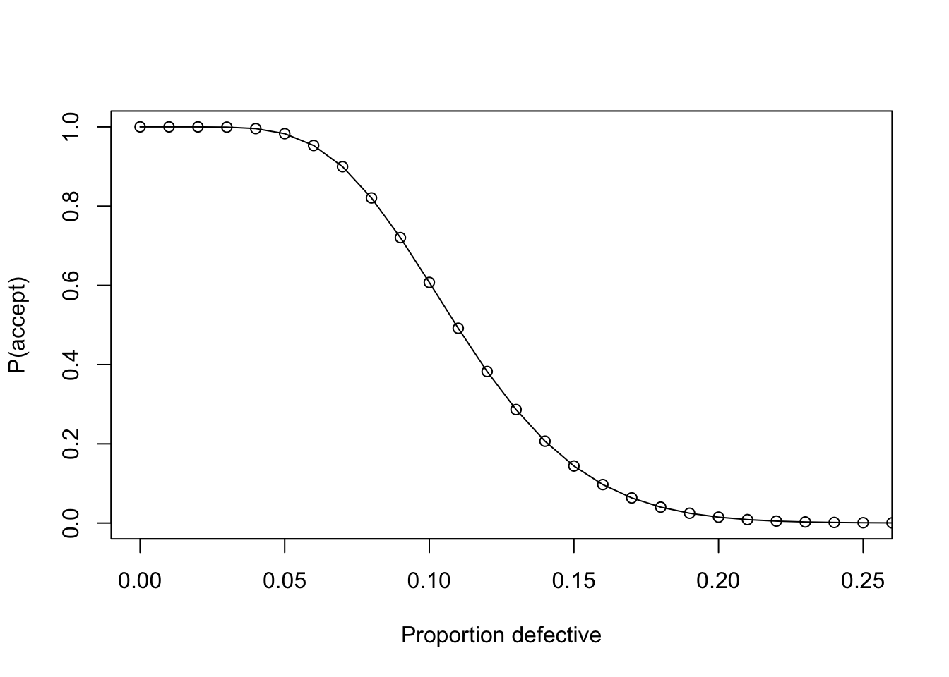
take a sample of 79 and reject when 9 items are defective
Variable Acceptance Sampling
specify:
- upper specification limit (USL)
and or:
- lower specification limit (LSL)
plan2 <- AcceptanceSampling::find.plan(
  PRP = c(0.06, 0.95),
  CRP = c(0.16, 0.10),
  type = "normal",
  s.type = "known"
)

plan2
## $n
## [1] 28
##
## $k
## [1] 1.243925
##
## $s.type
## [1] "known"proceed:
- take a sample of 28
- compute the mean
- compute LSL/USL - mean(sample) / sd
- compare accept if value above is greater 1.2439255
plan3 <- AcceptanceSampling::find.plan(
  PRP = c(0.06, 0.95),
  CRP = c(0.16, 0.10),
  type = "normal",
  s.type = "unknown"
)

plan3
## $n
## [1] 49
##
## $k
## [1] 1.245424
##
## $s.type
## [1] "unknown"proceed:
- take a sample of 49
- compute the mean
- compute LSL/USL - mean(sample) / sd(sample)
- compare accept if value above is greater 1.2454244
Note that sample size has increased because we do not know population sd and need to estimate it from the sample.