Moving from R to python - 5/7 - scikitlearn

- 1 of 7: IDE
- 2 of 7: pandas
- 3 of 7: matplotlib and seaborn
- 4 of 7: plotly
- 5 of 7: scikitlearn
- 6 of 7: advanced scikitlearn
- 7 of 7: automated machine learning
Table of Contents
scikitlearn
As I am starting out to read some scikitlearn tutorials I immedialtely spot some differences between scikitlearn and modelling in R.
- for
scikitlearndata needs to be numerical, so all categorical data needs to be converted to dummy variables first. - predictor and response variable have to be given in “matrix input”, there is no such thing as the formula input in
R - the nomenclature for the predictor matrix is
Xand for the responsey
Here we would like to perform a rather complex chain of steps.
Feature Engineeering
- Impute missing data
- Normalize numerical data
- Create dummy variables for categorical data
Modelling
- Fit a cross validated CART tree
- Use randomized parameter search to tune the tree
- Visualize the tree with the lowest error
- Visualize the ROC curve with SEM based on cv results
Sample Data
We have to provide the data in x,y format and have to convert all categoricals before hand. There are some sample datasets that come with scikitlearn but they are already pre-processed and contain no categorical variables. Here is an example
from sklearn import datasets

boston = datasets.load_boston()

print(boston.data)
print(boston.feature_names)
[[6.3200e-03 1.8000e+01 2.3100e+00 ... 1.5300e+01 3.9690e+02 4.9800e+00]
 [2.7310e-02 0.0000e+00 7.0700e+00 ... 1.7800e+01 3.9690e+02 9.1400e+00]
 [2.7290e-02 0.0000e+00 7.0700e+00 ... 1.7800e+01 3.9283e+02 4.0300e+00]
 ...
 [6.0760e-02 0.0000e+00 1.1930e+01 ... 2.1000e+01 3.9690e+02 5.6400e+00]
 [1.0959e-01 0.0000e+00 1.1930e+01 ... 2.1000e+01 3.9345e+02 6.4800e+00]
 [4.7410e-02 0.0000e+00 1.1930e+01 ... 2.1000e+01 3.9690e+02 7.8800e+00]]
['CRIM' 'ZN' 'INDUS' 'CHAS' 'NOX' 'RM' 'AGE' 'DIS' 'RAD' 'TAX' 'PTRATIO'
 'B' 'LSTAT']
Usually our datasets will not come that neatly prepared and we wont have numpy arrays but pandas dataframes. So alternatively we will get our datasets from seaborn
import seaborn as sns

df = sns.load_dataset('titanic')

df.head()
| survived | pclass | sex | age | sibsp | parch | fare | embarked | class | who | adult_male | deck | embark_town | alive | alone | |
|---|---|---|---|---|---|---|---|---|---|---|---|---|---|---|---|
| 0 | 0 | 3 | male | 22.0 | 1 | 0 | 7.2500 | S | Third | man | True | NaN | Southampton | no | False |
| 1 | 1 | 1 | female | 38.0 | 1 | 0 | 71.2833 | C | First | woman | False | C | Cherbourg | yes | False |
| 2 | 1 | 3 | female | 26.0 | 0 | 0 | 7.9250 | S | Third | woman | False | NaN | Southampton | yes | True |
| 3 | 1 | 1 | female | 35.0 | 1 | 0 | 53.1000 | S | First | woman | False | C | Southampton | yes | False |
| 4 | 0 | 3 | male | 35.0 | 0 | 0 | 8.0500 | S | Third | man | True | NaN | Southampton | no | True |
Investigating Data Set
df.dtypes
survived          int64
pclass            int64
sex              object
age             float64
sibsp             int64
parch             int64
fare            float64
embarked         object
class          category
who              object
adult_male         bool
deck           category
embark_town      object
alive            object
alone              bool
dtype: object
In R we would use summary to look at the number of levels of each factor variable. In python we would have to iterate over the categorical column names and use pd.Series.value_counts() which is a bit cumbersome. However this approach also gives us a bit more control than we have with summary() in R.
import pandas as pd
import numpy as np

def summary(df):

    print('categorical variables--------------------------------')

    for cat_var in df.select_dtypes(exclude = np.number).columns:

        counts = df[cat_var] \
            .value_counts( dropna= False ) \
            .to_frame()
        perc = df[cat_var] \
            .value_counts( dropna= False, normalize = True ) \
            .to_frame()

        print( df[cat_var].dtypes )
        print( counts.join(perc, lsuffix = '_n', rsuffix = '_perc' ) )
        print('')

    print('numerical variables----------------------------------')

    print( df.describe() )

summary(df)
categorical variables--------------------------------
object
        sex_n  sex_perc
male      577  0.647587
female    314  0.352413

object
     embarked_n  embarked_perc
S           644       0.722783
C           168       0.188552
Q            77       0.086420
NaN           2       0.002245

category
        class_n  class_perc
Third       491    0.551066
First       216    0.242424
Second      184    0.206510

object
       who_n  who_perc
man      537  0.602694
woman    271  0.304153
child     83  0.093154

bool
       adult_male_n  adult_male_perc
True            537         0.602694
False           354         0.397306

category
     deck_n  deck_perc
NaN     688   0.772166
C        59   0.066218
B        47   0.052750
D        33   0.037037
E        32   0.035915
A        15   0.016835
F        13   0.014590
G         4   0.004489

object
             embark_town_n  embark_town_perc
Southampton            644          0.722783
Cherbourg              168          0.188552
Queenstown              77          0.086420
NaN                      2          0.002245

object
     alive_n  alive_perc
no       549    0.616162
yes      342    0.383838

bool
       alone_n  alone_perc
True       537    0.602694
False      354    0.397306

numerical variables----------------------------------
         survived      pclass         age       sibsp       parch        fare
count  891.000000  891.000000  714.000000  891.000000  891.000000  891.000000
mean     0.383838    2.308642   29.699118    0.523008    0.381594   32.204208
std      0.486592    0.836071   14.526497    1.102743    0.806057   49.693429
min      0.000000    1.000000    0.420000    0.000000    0.000000    0.000000
25%      0.000000    2.000000   20.125000    0.000000    0.000000    7.910400
50%      0.000000    3.000000   28.000000    0.000000    0.000000   14.454200
75%      1.000000    3.000000   38.000000    1.000000    0.000000   31.000000
max      1.000000    3.000000   80.000000    8.000000    6.000000  512.329200
Some variables do have missing values which we have to impute.
Feature Engineering
Impute missing values
scikit-learn has some standard imputation methods like mean and median. There is a package called fancyimpute which can do knn imputing but has a huge list of required packages a lot of which require C++ compilation. We will therefore just use scikti-learn to start with. Like everything in scikitlearn we can only use it for numerical data.
Encode categorical variables
The imputation methods included in scikitlearn require numerical data. In order to use them for categorical data we have to assign a number to each level, apply the imputation method and then convert the numbers back to their corresponding levels. In the development version of scikitlearn we can find sklearn.preprocessing.CategoricalEncoder which apparently allows you to do easy onestep encoding and decoding. Then there is the package sklearn-pandas which also has a CategoricalEncoder and bridges both packages and is recommended on the pandas documentation homepage.
For exercise purposes however we will build our own Categorical Encoder. We will use pd.factorize() to convert the categorical columns to numerical, it returns a numerical array and an index which allows us to convert the array back to the categories. However there are some issues for this function.
NaNwill be represented with -1 in the array but dropped from the index in nonedtype == 'category'columns. Which makes recoding awkward- There is a bug for columns of
dtype == 'category'which only returns a numerical index and makes it impossible to recode back to categories from it. This bug will be fixed inpandas 0.23(as I am writing this the release version ispandas 0.19). This means we have to implement an ugly fix into our Encoder Class :-(. bugreport. NaNfor columns ofdtype == 'category'will not be encoded with a random integer within the range of the number of unique values. We need a consistent NaN integer for imputation.
Convert all none-numericals to dtype category
for col in df.select_dtypes(exclude = np.number).columns:
    df[col] = df[col].astype('object')
Categorical Encoder
class CategoricalEncoder:

    columns = list()
    dtypes = list()
    indeces = dict()


    def encode(self, df):

        # dont want the input object to change
        df = df.copy()

        self.columns = df.columns
        self.dtypes = df.dtypes

        assert len( df.select_dtypes(exclude = [np.number, 'object']).columns ) == 0 \
        , 'convert all none-numerical columns to object first'

        for col in df.select_dtypes(exclude = np.number):
            df[col], self.indeces[col] = pd.factorize(df[col])
            #df[col] = df[col].astype('int') ## array is returned as float :-(

        return df

    def recode(self, df):

        df = df.copy()

        assert any( df.columns == self.columns), 'columns do not match original dataframe'

        for col, ind in self.indeces.items():
            df[col] = [ np.nan if x == -1 else x for x in df[col] ] ## numpy converts array to float
            df[col] = [ ind[ int(x) ] if not np.isnan(x) else x for x in df[col] ] ## we need to convert back to int

        df = df.loc[:,self.columns]

        for col, dtype in zip(df.columns, self.dtypes):
            df[col] = df[col].astype(dtype.name)

        return df
Test Categorical Encoder
Encoder = CategoricalEncoder()

df_enc = Encoder.encode(df)

df_rec = Encoder.recode(df_enc)

assert df.equals(df_rec), 'Encoder does not recode correctly'
Impute
We will impute categroical with most frequent category and numericals with mean
from sklearn.preprocessing import Imputer

Encoder = CategoricalEncoder()

df_enc = Encoder.encode(df)

df_imp = df_enc.copy()

# numericals
col_num = df.select_dtypes(include = np.number).columns
Imputer_mean = Imputer(strategy = 'mean')
df_imp.loc[:, col_num] = Imputer_mean.fit_transform( df_imp.loc[:, col_num] )

# categoricals
col_cat = df.select_dtypes(exclude = np.number).columns
Imputer_freq = Imputer(strategy = 'most_frequent', missing_values = -1)
df_imp.loc[:, col_cat]  = Imputer_freq.fit_transform( df_imp.loc[:, col_cat] )

df_imp_rec = Encoder.recode(df_imp)

assert not df_imp_rec.isna().as_matrix().any()
assert df_imp_rec.shape == df.shape
c:\anaconda\envs\py36r343\lib\site-packages\ipykernel\__main__.py:21: FutureWarning: Method .as_matrix will be removed in a future version. Use .values instead.
Transforming numerical variables
Boxcox
Investigate distributions
from matplotlib import pyplot as plt
%matplotlib inline


def plot_hist_grid(df, x, y ):

    fig = plt.figure(figsize=(14, 12))

    for i, col in enumerate( df.select_dtypes( include = np.number).columns ):
        ax = fig.add_subplot(x,y,i+1)
        sns.distplot( df[col].dropna() )
        ax.set_title(col + ' distribution')

    fig.tight_layout() ## we need this so the histogram titles do not overlap


plot_hist_grid(df_imp_rec, 4, 2)
c:\anaconda\envs\py36r343\lib\site-packages\matplotlib\axes\_axes.py:6462: UserWarning: The 'normed' kwarg is deprecated, and has been replaced by the 'density' kwarg.
  warnings.warn("The 'normed' kwarg is deprecated, and has been "
c:\anaconda\envs\py36r343\lib\site-packages\matplotlib\axes\_axes.py:6462: UserWarning: The 'normed' kwarg is deprecated, and has been replaced by the 'density' kwarg.
  warnings.warn("The 'normed' kwarg is deprecated, and has been "
c:\anaconda\envs\py36r343\lib\site-packages\matplotlib\axes\_axes.py:6462: UserWarning: The 'normed' kwarg is deprecated, and has been replaced by the 'density' kwarg.
  warnings.warn("The 'normed' kwarg is deprecated, and has been "
c:\anaconda\envs\py36r343\lib\site-packages\matplotlib\axes\_axes.py:6462: UserWarning: The 'normed' kwarg is deprecated, and has been replaced by the 'density' kwarg.
  warnings.warn("The 'normed' kwarg is deprecated, and has been "
c:\anaconda\envs\py36r343\lib\site-packages\matplotlib\axes\_axes.py:6462: UserWarning: The 'normed' kwarg is deprecated, and has been replaced by the 'density' kwarg.
  warnings.warn("The 'normed' kwarg is deprecated, and has been "
c:\anaconda\envs\py36r343\lib\site-packages\matplotlib\axes\_axes.py:6462: UserWarning: The 'normed' kwarg is deprecated, and has been replaced by the 'density' kwarg.
  warnings.warn("The 'normed' kwarg is deprecated, and has been "
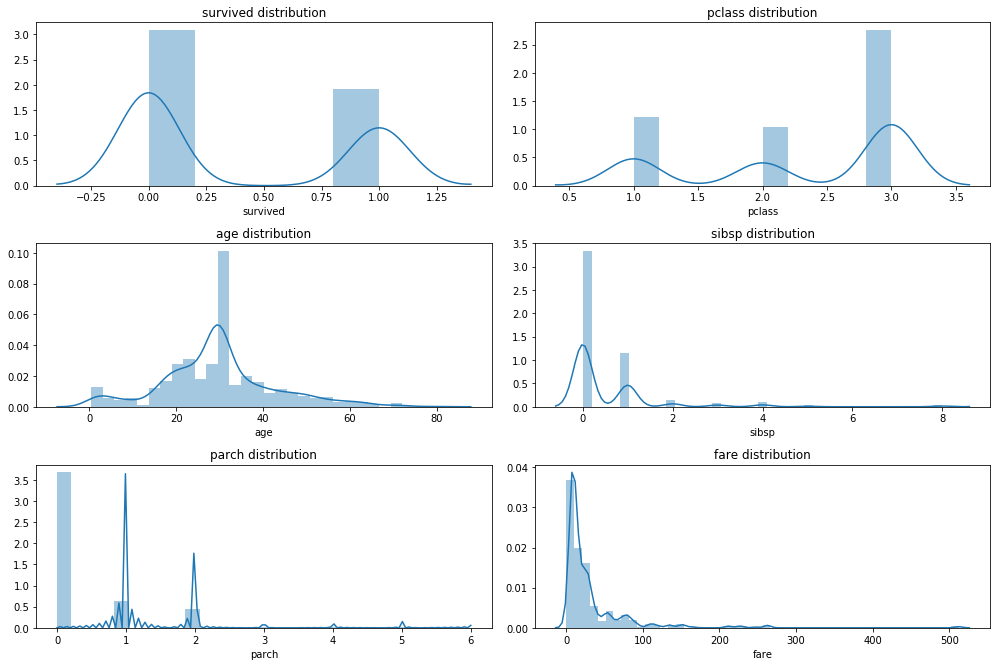
none of the numerical variables have a normal distribution, the best option here would be to use a Boxcox or a Yeo Johnson transformation if we plan on using a parametric model. Both algorithms return a lambda value that allows us to apply the same transformation to new data. Unfortunately the python implementations are a bit limited at the moment. There is sklearn.preprocessing.PowerTransformer in the newest development version of scikit-learn whis supports Boxcox transformations. Then there is scipy.stats.boxcox which is a bit cumbersome and requires a lot of manual work. Also Boxcox is a bit subborn and requires positive values. Probably feature processing is something you want to keep doing in R using recipes or caret.
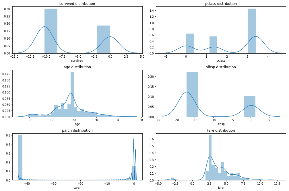
Apply Boxcox transformation
from scipy.stats import boxcox

df_trans = df_imp_rec.copy()

# boxcox needs values > 0
for col in df_imp_rec.select_dtypes(include = np.number).columns:
    df_trans[col] = df_trans[col] + 0.01

# scipy.stats implementaion cannot handle NA values
# df_trans = df_trans.dropna()

lambdas = dict()

for col in df_imp_rec.select_dtypes(include = np.number).columns:
    df_trans[col], lambdas[col] = boxcox(df_trans[col])

print( pd.Series(lambdas) )

plot_hist_grid(df_trans, 4, 2)

df_trans.describe()
age         0.822999
fare        0.180913
parch      -0.767354
pclass      1.774717
sibsp      -0.484927
survived   -0.312346
dtype: float64


c:\anaconda\envs\py36r343\lib\site-packages\matplotlib\axes\_axes.py:6462: UserWarning: The 'normed' kwarg is deprecated, and has been replaced by the 'density' kwarg.
  warnings.warn("The 'normed' kwarg is deprecated, and has been "
c:\anaconda\envs\py36r343\lib\site-packages\matplotlib\axes\_axes.py:6462: UserWarning: The 'normed' kwarg is deprecated, and has been replaced by the 'density' kwarg.
  warnings.warn("The 'normed' kwarg is deprecated, and has been "
c:\anaconda\envs\py36r343\lib\site-packages\matplotlib\axes\_axes.py:6462: UserWarning: The 'normed' kwarg is deprecated, and has been replaced by the 'density' kwarg.
  warnings.warn("The 'normed' kwarg is deprecated, and has been "
c:\anaconda\envs\py36r343\lib\site-packages\matplotlib\axes\_axes.py:6462: UserWarning: The 'normed' kwarg is deprecated, and has been replaced by the 'density' kwarg.
  warnings.warn("The 'normed' kwarg is deprecated, and has been "
c:\anaconda\envs\py36r343\lib\site-packages\matplotlib\axes\_axes.py:6462: UserWarning: The 'normed' kwarg is deprecated, and has been replaced by the 'density' kwarg.
  warnings.warn("The 'normed' kwarg is deprecated, and has been "
c:\anaconda\envs\py36r343\lib\site-packages\matplotlib\axes\_axes.py:6462: UserWarning: The 'normed' kwarg is deprecated, and has been replaced by the 'density' kwarg.
  warnings.warn("The 'normed' kwarg is deprecated, and has been "
| survived | pclass | age | sibsp | parch | fare | |
|---|---|---|---|---|---|---|
| count | 891.000000 | 891.000000 | 891.000000 | 891.000000 | 891.000000 | 891.000000 |
| mean | -6.336364 | 2.172058 | 18.275863 | -11.647712 | -32.911718 | 3.910416 |
| std | 5.011771 | 1.456663 | 7.261755 | 8.111499 | 18.608375 | 1.965039 |
| min | -10.289796 | 0.010039 | -0.608408 | -17.176613 | -43.335522 | -3.124792 |
| 25% | -10.289796 | 1.381702 | 14.257979 | -17.176613 | -43.335522 | 2.510059 |
| 50% | -10.289796 | 3.419353 | 18.590518 | -17.176613 | -43.335522 | 3.435259 |
| 75% | 0.009935 | 3.419353 | 21.455870 | 0.009926 | -43.335522 | 4.761225 |
| max | 0.009935 | 3.419353 | 43.544598 | 1.310322 | 0.974077 | 11.561796 |
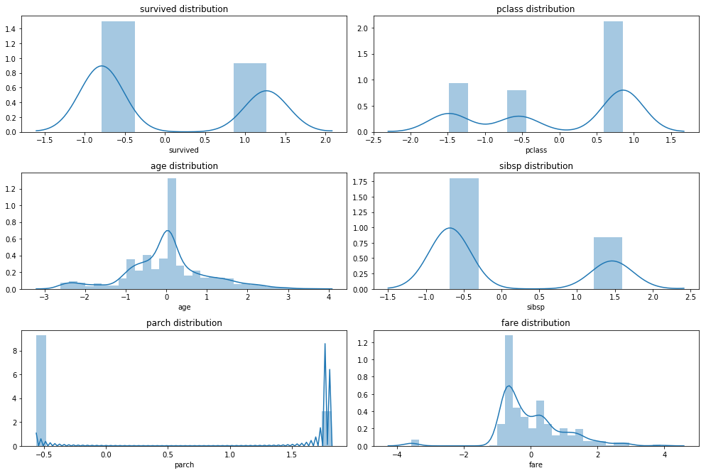
Scale
from sklearn.preprocessing import StandardScaler

Scaler = StandardScaler()

cols_num = df_trans.select_dtypes(include = np.number).columns
df_trans.loc[:,cols_num] = Scaler.fit_transform( df_trans.loc[:,cols_num] )

plot_hist_grid(df_trans, 4, 2)
c:\anaconda\envs\py36r343\lib\site-packages\matplotlib\axes\_axes.py:6462: UserWarning: The 'normed' kwarg is deprecated, and has been replaced by the 'density' kwarg.
  warnings.warn("The 'normed' kwarg is deprecated, and has been "
c:\anaconda\envs\py36r343\lib\site-packages\matplotlib\axes\_axes.py:6462: UserWarning: The 'normed' kwarg is deprecated, and has been replaced by the 'density' kwarg.
  warnings.warn("The 'normed' kwarg is deprecated, and has been "
c:\anaconda\envs\py36r343\lib\site-packages\matplotlib\axes\_axes.py:6462: UserWarning: The 'normed' kwarg is deprecated, and has been replaced by the 'density' kwarg.
  warnings.warn("The 'normed' kwarg is deprecated, and has been "
c:\anaconda\envs\py36r343\lib\site-packages\matplotlib\axes\_axes.py:6462: UserWarning: The 'normed' kwarg is deprecated, and has been replaced by the 'density' kwarg.
  warnings.warn("The 'normed' kwarg is deprecated, and has been "
c:\anaconda\envs\py36r343\lib\site-packages\matplotlib\axes\_axes.py:6462: UserWarning: The 'normed' kwarg is deprecated, and has been replaced by the 'density' kwarg.
  warnings.warn("The 'normed' kwarg is deprecated, and has been "
c:\anaconda\envs\py36r343\lib\site-packages\matplotlib\axes\_axes.py:6462: UserWarning: The 'normed' kwarg is deprecated, and has been replaced by the 'density' kwarg.
  warnings.warn("The 'normed' kwarg is deprecated, and has been "
Final feature selection
Finally we have some duplicate information in our dataframe which we will drop.
df_fin = df_trans.drop(['survived','pclass'], axis = 1)
Encoding Categorical variables
In R we did not have to worry much about encoding categorical data it would usually be taken care of by most modelling algorithms. In python we have to do this manually.
There is an excellent guide from which I will try to replicate some of the examples. Digging into the topic a bit I also learned that there are more encoding techniques for categorical variabels than just the regular dummy encoding which is used by R as the gold standard. There is also one hot encoding which creates for a categorical variable with k categories k binary columns (compared to k-1 columns for dummy encoding). Beyond those two methods there are plenty more as described in this article. For these types of encodings the categorical values will be replaced with the summarized values of the response variable of all observations from the same category such as the sum or the mean. This is similar to the weight of evidence encoding which is commonly used when developing credit risk score cards with logistic regression.
Returning to the samply data we can see that we have duplicated information such as the columns sex, who, and adult_male. Here we will select only one of each of those and prefer categorical string encoding over variables that already have numerical or binary encoding.
Create dummy variables
There is no algorithm in scikitlearn that creates dummy variables we therefore need to borrow this functionality from pandas.
df_dum = pd.get_dummies(df_fin
               , drop_first = True ## k-1 dummy variables
              )

df_dum.head()
| age | sibsp | parch | fare | sex_male | embarked_Q | embarked_S | class_Second | class_Third | who_man | ... | deck_B | deck_C | deck_D | deck_E | deck_F | deck_G | embark_town_Queenstown | embark_town_Southampton | alive_yes | alone_True | |
|---|---|---|---|---|---|---|---|---|---|---|---|---|---|---|---|---|---|---|---|---|---|
| 0 | -0.553605 | 1.437981 | -0.560482 | -0.776991 | 1 | 0 | 1 | 0 | 1 | 1 | ... | 0 | 1 | 0 | 0 | 0 | 0 | 0 | 1 | 0 | 0 |
| 1 | 0.656833 | 1.437981 | -0.560482 | 1.284747 | 0 | 0 | 0 | 0 | 0 | 0 | ... | 0 | 1 | 0 | 0 | 0 | 0 | 0 | 0 | 1 | 0 |
| 2 | -0.239527 | -0.681996 | -0.560482 | -0.711671 | 0 | 0 | 1 | 0 | 1 | 0 | ... | 0 | 1 | 0 | 0 | 0 | 0 | 0 | 1 | 1 | 1 |
| 3 | 0.438158 | 1.437981 | -0.560482 | 0.968817 | 0 | 0 | 1 | 0 | 0 | 0 | ... | 0 | 1 | 0 | 0 | 0 | 0 | 0 | 1 | 1 | 0 |
| 4 | 0.438158 | -0.681996 | -0.560482 | -0.700078 | 1 | 0 | 1 | 0 | 1 | 1 | ... | 0 | 1 | 0 | 0 | 0 | 0 | 0 | 1 | 0 | 1 |
5 rows × 22 columns
Fitting a decision tree
We will fit an examplatory decision tree to the data. Not because it is the best model to use here but because decision trees can easily be visualised graphically and it is a good exercise to try that out. We will perform a 10 x 10-fold cross validation and a randomized parameter search.
Hyperparameter Tuning
Traditionally one would use a grid search of all possible hyperparameter combinations in order to optimize model performance. Recently a number of more efficient algorithms have been developed.
- The submodel trick: For some ensemble methods one of the tuning parameters usually reflects the number of contrbuting models such as the number of trees in a random forest. In order to train a forest with 1000 trees we have in the process also to train models for all numbers of trees between 1:1000. The submodel trick simpoly implies that we are saving these intermediary models for evaluation. The submodel trick is used by many model implementations in the
caretpackage. Usually the implementation of the submodel trick outweighs the benefits of the other hyperparameter optimizations strategies. - Adaptive Resampling: In order to validate model performance we have to use k-fold cross validation, k usually depends on the size and variance in the data. Sometimes variance in the data is so high that each k-fold split of the data gives us different results, so we have to perform x times k-fold cross validaztion. For most of the hyperparameter combinations in a grid search however we can probably already predict after analysing just a few cross validation pairs that they will not produce better results than the best combination that we have found so far. Max Kuhn has presented to techniques for prediciting model performance after only a few resampling rounds in his 2014 paper which have been experimentally implemented in
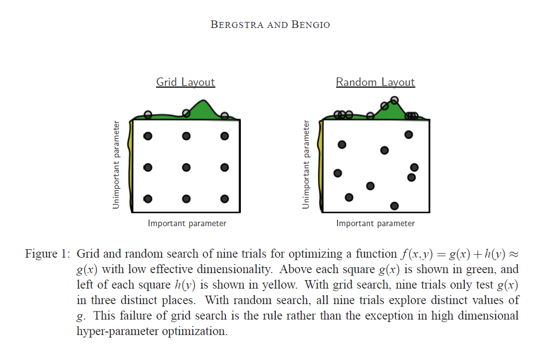
caret. - Randomized Search: Experience in hyperparamter tuning has shown that only a few of the tunable parameters of a model actually have an influence on model performance. Which those parameters are however is largely influenced by the dataset. In a case where the model performance is largely dominated by a single parameter a randomized search covers a larger range of that parameter than a grid search as demonstrated in this [paper] and exemplified in the illustration below. (http://www.jmlr.org/papers/volume13/bergstra12a/bergstra12a.pdf). Randomized search is implemented in
caretas well as inscikitlearn
Randomized parameter search
Instead of specifiying a range for certain parameters we will provide a distribution to sample from an the number of iterations the algorithm should use. We can get the distributions from the scipy.stats package. Since we have no prior knowledge about which distributions to chose we simply chose stats.randint for discrete values and stats.uniform for contineous values.
from sklearn.tree import DecisionTreeClassifier
from sklearn.model_selection import RandomizedSearchCV
from sklearn.model_selection import RepeatedKFold
from scipy import stats


clf = DecisionTreeClassifier()

param_dist = {'min_samples_split': stats.randint(2,250)
             , 'min_samples_leaf': stats.randint(1,500)
             , 'min_impurity_decrease' : stats.uniform(0,1)
             , 'max_features': stats.uniform(0,1) }

n_iter = 2500

random_search = RandomizedSearchCV(clf
                                   , param_dist
                                   , n_iter = n_iter
                                   , scoring = 'roc_auc'
                                   , cv = RepeatedKFold( n_splits = 10, n_repeats = 10 )
                                   , verbose = True
                                   , n_jobs = 4 ## parallel processing
                                   , return_train_score = True
                                  )

x = df_dum.drop('alive_yes', axis = 1)
y = df_dum['alive_yes']

random_search.fit(x,y)
Fitting 100 folds for each of 2500 candidates, totalling 250000 fits


[Parallel(n_jobs=4)]: Done 142 tasks      | elapsed:    4.4s
[Parallel(n_jobs=4)]: Done 7538 tasks      | elapsed:   20.7s
[Parallel(n_jobs=4)]: Done 20038 tasks      | elapsed:   50.3s
[Parallel(n_jobs=4)]: Done 37538 tasks      | elapsed:  1.4min
[Parallel(n_jobs=4)]: Done 60038 tasks      | elapsed:  2.3min
[Parallel(n_jobs=4)]: Done 87538 tasks      | elapsed:  3.1min
[Parallel(n_jobs=4)]: Done 120038 tasks      | elapsed:  4.2min
[Parallel(n_jobs=4)]: Done 157538 tasks      | elapsed:  5.3min
[Parallel(n_jobs=4)]: Done 200038 tasks      | elapsed:  6.7min
[Parallel(n_jobs=4)]: Done 247538 tasks      | elapsed:  8.2min
[Parallel(n_jobs=4)]: Done 250000 out of 250000 | elapsed:  8.3min finished


RandomizedSearchCV(cv=<sklearn.model_selection._split.RepeatedKFold object at 0x0000026252BAB048>,
          error_score='raise',
          estimator=DecisionTreeClassifier(class_weight=None, criterion='gini', max_depth=None,
            max_features=None, max_leaf_nodes=None,
            min_impurity_decrease=0.0, min_impurity_split=None,
            min_samples_leaf=1, min_samples_split=2,
            min_weight_fraction_leaf=0.0, presort=False, random_state=None,
            splitter='best'),
          fit_params=None, iid=True, n_iter=2500, n_jobs=4,
          param_distributions={'max_features': <scipy.stats._distn_infrastructure.rv_frozen object at 0x0000026252BB9EB8>, 'min_samples_leaf': <scipy.stats._distn_infrastructure.rv_frozen object at 0x0000026252B4B898>, 'min_samples_split': <scipy.stats._distn_infrastructure.rv_frozen object at 0x00000262515C0208>, 'min_impurity_decrease': <scipy.stats._distn_infrastructure.rv_frozen object at 0x0000026252BB9BE0>},
          pre_dispatch='2*n_jobs', random_state=None, refit=True,
          return_train_score=True, scoring='roc_auc', verbose=True)
res = pd.DataFrame( random_search.cv_results_ )

res.sort_values('rank_test_score').head(10)
| mean_fit_time | mean_score_time | mean_test_score | mean_train_score | param_max_features | param_min_impurity_decrease | param_min_samples_leaf | param_min_samples_split | params | rank_test_score | ... | split98_test_score | split98_train_score | split99_test_score | split99_train_score | split9_test_score | split9_train_score | std_fit_time | std_score_time | std_test_score | std_train_score | |
|---|---|---|---|---|---|---|---|---|---|---|---|---|---|---|---|---|---|---|---|---|---|
| 1128 | 0.003643 | 0.001576 | 0.849557 | 0.850829 | 0.922112 | 0.00837461 | 83 | 31 | {'max_features': 0.9221122085261761, 'min_samp... | 1 | ... | 0.828734 | 0.819121 | 0.901695 | 0.850536 | 0.863777 | 0.854140 | 0.006607 | 0.004447 | 0.041007 | 0.011566 |
| 1633 | 0.003828 | 0.001679 | 0.847263 | 0.851479 | 0.768034 | 0.006899 | 29 | 222 | {'max_features': 0.7680338558114431, 'min_samp... | 2 | ... | 0.885823 | 0.849771 | 0.888136 | 0.839672 | 0.846749 | 0.834493 | 0.002111 | 0.002052 | 0.037894 | 0.010166 |
| 2212 | 0.003988 | 0.001859 | 0.844536 | 0.849014 | 0.93337 | 0.0106538 | 83 | 63 | {'max_features': 0.9333697771766865, 'min_samp... | 3 | ... | 0.882846 | 0.851963 | 0.901695 | 0.850536 | 0.863777 | 0.854140 | 0.001951 | 0.002024 | 0.043665 | 0.014672 |
| 753 | 0.003812 | 0.001781 | 0.824468 | 0.835190 | 0.454209 | 0.00670731 | 54 | 112 | {'max_features': 0.4542091923263467, 'min_samp... | 4 | ... | 0.882846 | 0.857641 | 0.854237 | 0.798901 | 0.865067 | 0.859434 | 0.007824 | 0.004666 | 0.051183 | 0.024695 |
| 1984 | 0.004388 | 0.001939 | 0.824068 | 0.829957 | 0.625724 | 0.000519658 | 150 | 142 | {'max_features': 0.6257243210055624, 'min_samp... | 5 | ... | 0.875541 | 0.848625 | 0.877119 | 0.836702 | 0.870485 | 0.816932 | 0.003914 | 0.002773 | 0.045516 | 0.022024 |
| 19 | 0.003757 | 0.001928 | 0.821358 | 0.830195 | 0.749645 | 0.0125087 | 74 | 176 | {'max_features': 0.7496448239892235, 'min_samp... | 6 | ... | 0.828734 | 0.819121 | 0.897740 | 0.847374 | 0.793344 | 0.778700 | 0.006965 | 0.005535 | 0.052542 | 0.023273 |
| 1201 | 0.003417 | 0.001224 | 0.811420 | 0.813680 | 0.854926 | 0.0129389 | 135 | 171 | {'max_features': 0.8549262726597407, 'min_samp... | 7 | ... | 0.828734 | 0.819121 | 0.866102 | 0.815483 | 0.837461 | 0.818296 | 0.006255 | 0.003975 | 0.048909 | 0.017295 |
| 841 | 0.002967 | 0.001803 | 0.810736 | 0.812231 | 0.837255 | 0.0214463 | 96 | 61 | {'max_features': 0.8372554895640392, 'min_samp... | 8 | ... | 0.828734 | 0.819121 | 0.832203 | 0.774712 | 0.837461 | 0.818296 | 0.006010 | 0.004641 | 0.044853 | 0.017689 |
| 998 | 0.003285 | 0.001589 | 0.807049 | 0.808691 | 0.792215 | 0.0331625 | 47 | 234 | {'max_features': 0.7922151495137242, 'min_samp... | 9 | ... | 0.828734 | 0.819121 | 0.866102 | 0.815483 | 0.793344 | 0.778700 | 0.006297 | 0.004970 | 0.047764 | 0.018487 |
| 1892 | 0.004287 | 0.001516 | 0.805288 | 0.806958 | 0.729024 | 0.0344067 | 126 | 116 | {'max_features': 0.7290237550895209, 'min_samp... | 10 | ... | 0.828734 | 0.819121 | 0.866102 | 0.815483 | 0.837461 | 0.818296 | 0.008426 | 0.004454 | 0.052977 | 0.018888 |
10 rows × 214 columns
from matplotlib import cm

params = ['param_max_features'
         , 'param_min_impurity_decrease'
         , 'param_min_samples_split']


cmap = cm.get_cmap('Dark2')

fig = plt.figure( figsize=(14, 12) )

for i, param in enumerate(params):

    ax = fig.add_subplot(2,2,i+1)

    sns.regplot( x = param
               , y = 'mean_test_score'
               , data = res # res.query('mean_test_score > 0.5')
               , scatter_kws = { 'color' :cmap(i) }
               , fit_reg = False
             )


    ax.set_title(param)


fig.tight_layout() ## we need this so the histogram titles do not overlap
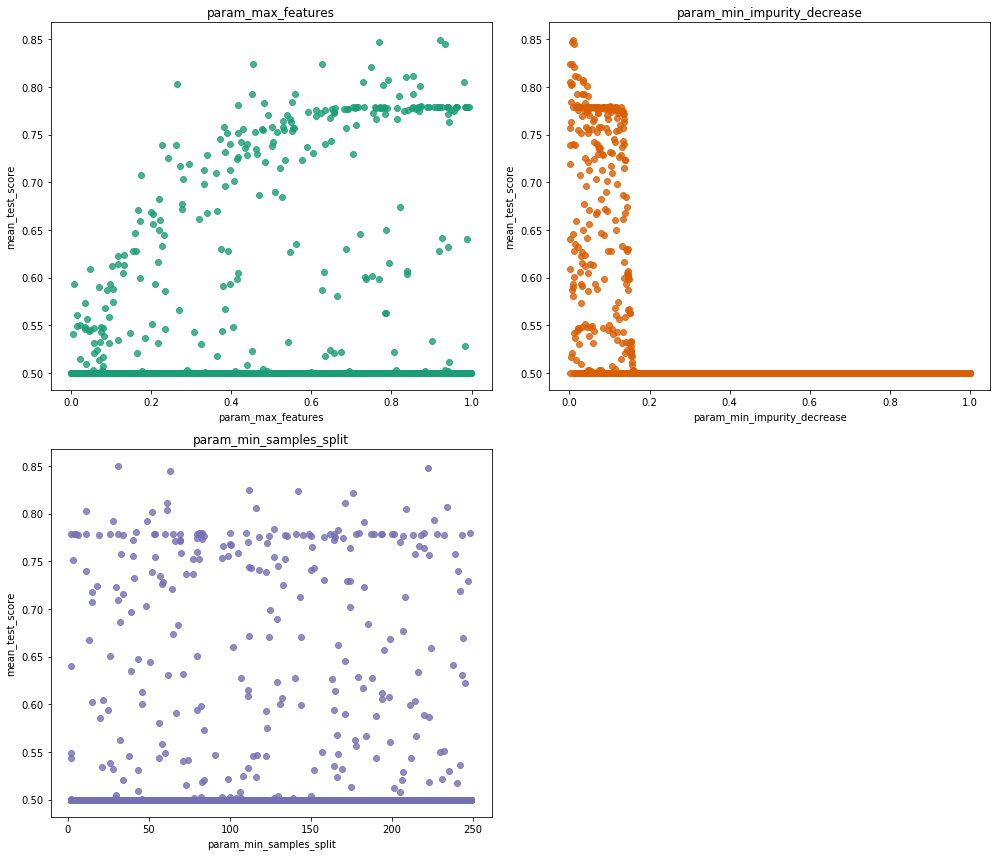
We can see that we only have a very narrow range for which min_impurity_decrease is optimal, the param_max_features value probably should be kept at maximum and min_samples_split probably does not have a large influence on performance.
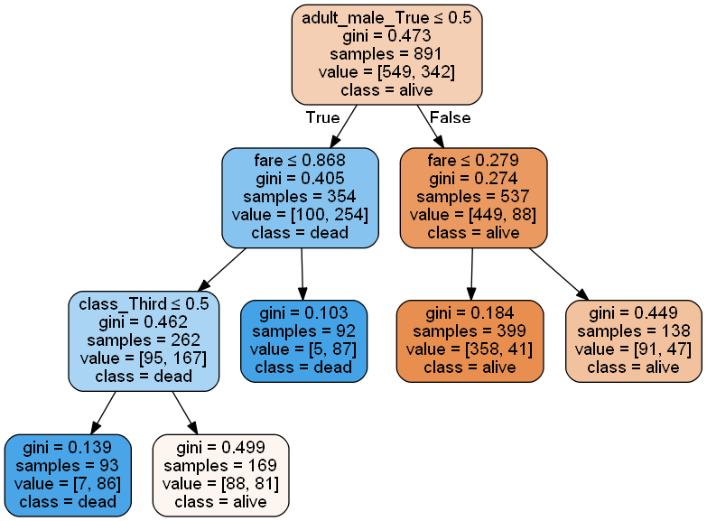
Visualize Tree
Scikitlearn allows us to export a decision tree graphic in GraphViz dot language format. We can interpret this format using PyDotPlus. In order for this to work we need to download and install GraphViz and put the installation folder into the PATH variable as well as pip installing the graphviz python package. See the documentation for installation instructions. For this tree we loose some of the interpretability because of the scaling and the boxcox transformation.
tree = random_search.best_estimator_

from sklearn.externals.six import StringIO
from IPython.display import Image
from sklearn.tree import export_graphviz
import pydotplus

dot_data = StringIO()

export_graphviz(tree
                , out_file = dot_data
                , filled = True
                , rounded = True
                , special_characters = True
                , feature_names = x.columns
                , class_names = ['alive', 'dead'] )

graph = pydotplus.graph_from_dot_data( dot_data.getvalue() )

Image( graph.create_png() )
Feature Importance
pd.DataFrame({ 'features' : x.columns, 'importance': tree.feature_importances_}) \
    .sort_values('importance', ascending = False)
| features | importance | |
|---|---|---|
| 11 | adult_male_True | 0.730129 |
| 3 | fare | 0.136980 |
| 8 | class_Third | 0.132890 |
| 0 | age | 0.000000 |
| 12 | deck_B | 0.000000 |
| 19 | embark_town_Southampton | 0.000000 |
| 18 | embark_town_Queenstown | 0.000000 |
| 17 | deck_G | 0.000000 |
| 16 | deck_F | 0.000000 |
| 15 | deck_E | 0.000000 |
| 14 | deck_D | 0.000000 |
| 13 | deck_C | 0.000000 |
| 10 | who_woman | 0.000000 |
| 1 | sibsp | 0.000000 |
| 9 | who_man | 0.000000 |
| 7 | class_Second | 0.000000 |
| 6 | embarked_S | 0.000000 |
| 5 | embarked_Q | 0.000000 |
| 4 | sex_male | 0.000000 |
| 2 | parch | 0.000000 |
| 20 | alone_True | 0.000000 |
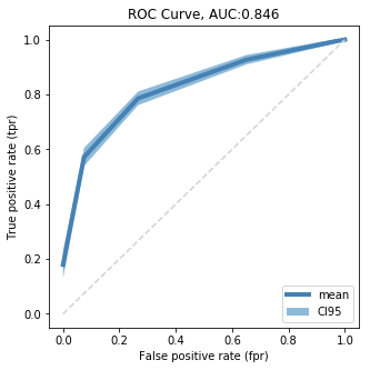
ROC Curve
Lets visualize a ROC curve for the tree with the best parameters and all 10x10x cross validation sets. Loosely inspired by this example code
Get tpr, fpr values for cv pairs
from sklearn.model_selection import cross_val_score
import sklearn

cv = sklearn.model_selection.RepeatedKFold(10,10)

tree = random_search.best_estimator_

results_df = pd.DataFrame( columns = ['fold', 'fpr', 'tpr', 'thresh', 'auc'] )


for i, split in enumerate(cv.split(x,y)):

    train, test = split

    tree = tree.fit(x.loc[train,:], y[train])

    pred_arr =  tree.predict_proba( x.loc[test,:] )
    # predict outputs probability for positive and negative outcome
    pred =  pd.DataFrame(pred_arr).loc[:,1]

    real = y[test]

    fpr, tpr, thresh = sklearn.metrics.roc_curve( y_true = real, y_score = pred)

    auc = sklearn.metrics.auc(fpr, tpr)

    rocs = pd.DataFrame({'fold': i, 'fpr': fpr, 'tpr': tpr , 'thresh': thresh, 'auc': auc})

    results_df = pd.concat([results_df, rocs], axis = 0)

    results_df_reind = results_df.reset_index( inplace = False ) \
        .rename(columns = {'index':'seq'})

results_df_reind.head(20)
c:\anaconda\envs\py36r343\lib\site-packages\ipykernel\__main__.py:30: FutureWarning: Sorting because non-concatenation axis is not aligned. A future version
of pandas will change to not sort by default.

To accept the future behavior, pass 'sort=False'.

To retain the current behavior and silence the warning, pass 'sort=True'.
| seq | auc | fold | fpr | thresh | tpr | |
|---|---|---|---|---|---|---|
| 0 | 0 | 0.800735 | 0 | 0.000000 | 1.957576 | 0.000000 |
| 1 | 1 | 0.800735 | 0 | 0.032787 | 0.957576 | 0.517241 |
| 2 | 2 | 0.800735 | 0 | 0.229508 | 0.490323 | 0.689655 |
| 3 | 3 | 0.800735 | 0 | 0.426230 | 0.352459 | 0.827586 |
| 4 | 4 | 0.800735 | 0 | 1.000000 | 0.100279 | 1.000000 |
| 5 | 0 | 0.877193 | 1 | 0.000000 | 0.945455 | 0.531250 |
| 6 | 1 | 0.877193 | 1 | 0.105263 | 0.475309 | 0.656250 |
| 7 | 2 | 0.877193 | 1 | 0.245614 | 0.325203 | 0.875000 |
| 8 | 3 | 0.877193 | 1 | 1.000000 | 0.105114 | 1.000000 |
| 9 | 0 | 0.887881 | 2 | 0.000000 | 0.946746 | 0.464286 |
| 10 | 1 | 0.887881 | 2 | 0.213115 | 0.472973 | 0.857143 |
| 11 | 2 | 0.887881 | 2 | 0.377049 | 0.357143 | 0.928571 |
| 12 | 3 | 0.887881 | 2 | 1.000000 | 0.108635 | 1.000000 |
| 13 | 0 | 0.845894 | 3 | 0.000000 | 1.951515 | 0.000000 |
| 14 | 1 | 0.845894 | 3 | 0.019231 | 0.951515 | 0.432432 |
| 15 | 2 | 0.845894 | 3 | 0.115385 | 0.452229 | 0.702703 |
| 16 | 3 | 0.845894 | 3 | 0.288462 | 0.338710 | 0.837838 |
| 17 | 4 | 0.845894 | 3 | 1.000000 | 0.098315 | 1.000000 |
| 18 | 0 | 0.916837 | 4 | 0.000000 | 0.944099 | 0.525000 |
| 19 | 1 | 0.916837 | 4 | 0.081633 | 0.442308 | 0.825000 |
results_gr = results_df_reind.groupby('seq') \
    .agg({'tpr':['mean', 'sem']
          , 'fpr':['mean', 'sem']
          , 'thresh':'mean'
          } )

results_gr
| tpr | fpr | thresh | |||
|---|---|---|---|---|---|
| mean | sem | mean | sem | mean | |
| seq | |||||
| 0 | 0.178960 | 0.024876 | 0.000000 | 0.000000 | 1.577290 |
| 1 | 0.571897 | 0.016556 | 0.074479 | 0.007452 | 0.794128 |
| 2 | 0.785816 | 0.012450 | 0.266459 | 0.018996 | 0.430423 |
| 3 | 0.926658 | 0.008574 | 0.650176 | 0.033806 | 0.244318 |
| 4 | 0.993480 | 0.003889 | 0.965127 | 0.019782 | 0.116393 |
| 5 | 1.000000 | 0.000000 | 1.000000 | 0.000000 | 0.104326 |
Plot ROC Curve
cmap = cm.get_cmap('Dark2')

fig = plt.figure( figsize=(5, 5) )


plt.plot( results_gr.fpr['mean'], results_gr.tpr['mean']
         , color = 'steelblue'
         , lw = 4
         , label = 'mean')

plt.plot( [0,1],[0,1]
         , color = 'lightgrey'
         , linestyle='--' )

plt.fill_between( results_gr.fpr['mean']
                 , results_gr.tpr['mean'] - 2 * results_gr.tpr['sem']
                 , results_gr.tpr['mean'] + 2 * results_gr.tpr['sem']
                 , alpha = 0.5
                 , label = 'CI95' )

plt.xlabel('False positive rate (fpr)')
plt.ylabel('True positive rate (tpr)')
plt.legend( loc = 'lower right')
plt.title('ROC Curve, AUC:{}'.format( results_df_reind.auc.unique().mean().round(3) ))

plt.show()